
Floating Point
Table of Contents
- A fixed set of points
- Floating the point
- The map
- The edges of the map
- The field guide
- float64
- float32, and the format hiding inside it
- float16
- bfloat16
- Rounding
- Where arithmetic goes wrong
- The little epsilons, explained
- Why smaller floats
- The update that vanished
- Loss scaling
- FP8
- The outlier problem
- Microscaling
- Training at 4 bits
- The other grids
- The whole family on one sheet
- Where the bytes live
- Hardware truth
- The contract
- Where this came from
- Build it yourself
- What you can now say
- Try it yourself
- References
Run this anywhere:
>>> 0.1 + 0.2
0.30000000000000004
>>> 0.1 + 0.2 == 0.3
False
And in real training runs, this happens:
step 39,998   loss 2.41
step 39,999   loss 2.40
step 40,000   loss nan
Both outputs have the same cause: the way computers store numbers. By the end of this page you will be able to predict both, explain them to someone else, and read a line like "MXFP4, E2M1, block 32, E8M0 scale" part by part. No prior knowledge is assumed. Every measured number on this page comes from a small script you can run, linked where the number appears, measured on an Apple M3 Max with torch 2.11.0 [1].
A fixed set of points
A computer stores a number in a fixed number of bits. Each bit has 2 states, so 32 bits can form 2 x 2 x ... x 2 = 2^32 = 4,294,967,296 different patterns. A number format assigns one number to each pattern. So for a 32-bit machine only those 4,294,967,296 numbers exist; anything else you compute is moved to the nearest one of them, and the distance moved is the rounding error. A format is exactly this: a choice of which numbers get a pattern. This page is about how that choice is made.
First, see the size of the problem. Between 1 and 2 there are infinitely many numbers. Zoom in anywhere and you find more. The line is never empty, at any depth. A format is a finite list of points. So almost no computed number is on the list, and almost every operation ends with a move to the nearest point: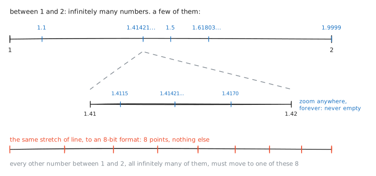
The simplest choice is equal spacing: 0, 1, 2, 3, and so on, the same distance 1 between every pair of neighbors. That is what integers are, and for counting it works. Now take two numbers that one real neural network produced in one training step: an activation of 10.5 (a value flowing through the network) and a gradient of 0.0000004 (a value that steers learning). Store both with equally spaced points: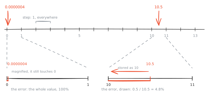
Those 2 numbers are not invented. They come from 1 training step of a small network, and this page keeps returning to that step, so here it is, drawn: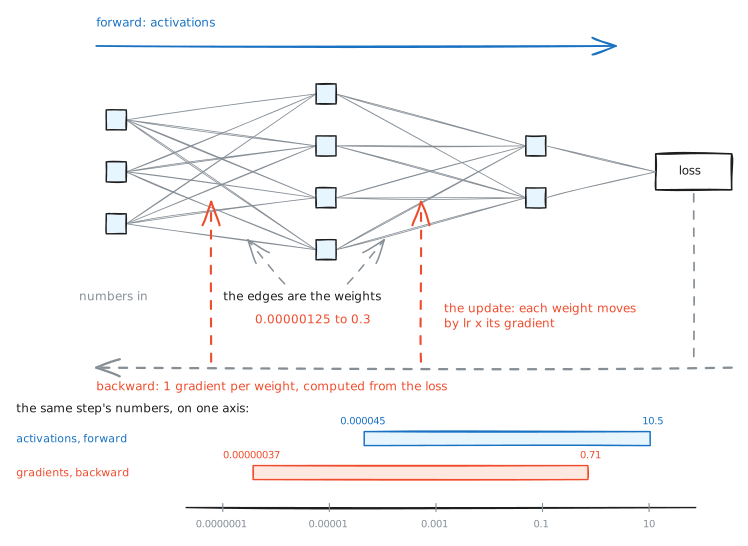
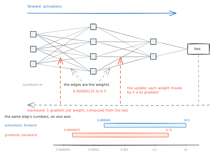
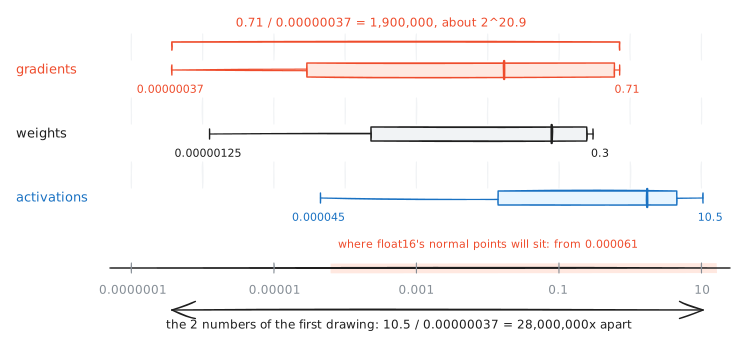
3 kinds of numbers move in that step. Activations are the values flowing forward through the layers. Weights are the numbers the network is learning; multiplying by them is what a layer does. Gradients are computed backward from the loss, 1 for every weight: each one says how much that weight should move. Train the network for a few seconds and measure all 3: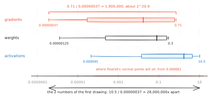
p1_where_numbers_live.py the proof, ready to read or run
download and run it# where a real network's numbers live.
#
# train a small mlp for about 2 seconds, then measure the spans of
# its weights, gradients, and activations in a single step. the
# point: one model needs numbers about 9 orders of magnitude apart
# at the same moment, so no uniform grid can serve both ends.
import math
import torch, torch.nn as nn
torch.manual_seed(0) # same numbers on every run
net = nn.Sequential(nn.Linear(64, 256), nn.ReLU(),
nn.Linear(256, 256), nn.ReLU(), nn.Linear(256, 1))
opt = torch.optim.Adam(net.parameters(), lr=1e-3)
X = torch.randn(4096, 64); y = (X[:, :3].prod(1, keepdim=True) * 10)
for step in range(300):
opt.zero_grad()
loss = ((net(X) - y) ** 2).mean()
loss.backward(); opt.step()
# flatten every weight and every gradient into one tensor each,
# plus the activations flowing out of the middle linear layer
tensors = {"weights": torch.cat([p.detach().flatten() for p in net.parameters()]),
"grads": torch.cat([p.grad.flatten() for p in net.parameters()])}
with torch.no_grad():
a = net[1](net[0](X)) # first linear, then its relu
tensors["activations"] = net[2](a).flatten()
print(f"final loss {loss.item():.3f}")
for name, t in tensors.items():
nz = t[t != 0].abs() # zeros have no magnitude to place
q = torch.quantile(nz, torch.tensor([0.001, 0.5, 0.999]))
print(f"{name:12s} |min..max| {nz.min():.2e} .. {nz.max():.2e} "
f"p0.1/median/p99.9 {q[0]:.2e} / {q[1]:.2e} / {q[2]:.2e}")
span = tensors["grads"].abs()[tensors["grads"] != 0]
print(f"gradient span: {math.log2(span.max() / span.min()):.1f} powers of two "
f"in one tensor family, this small a net, this early")
# the histogram behind the drawn silhouettes: what share of each
# tensor lands in each power-of-10 decade
print("\ndecade histogram (percent of values per log10 decade; "
"the drawn silhouettes):")
edges = list(range(-8, 2))
for name, t in tensors.items():
nz = t[t != 0].abs().log10()
counts = [(100.0 * ((nz >= a) & (nz < a + 1)).sum() / nz.numel())
for a in edges]
row = " ".join(f"{c:4.1f}" for c in counts)
print(f"{name:12s} [{edges[0]}..{edges[-1] + 1}] {row}")
# the run prints (seeded, so the same everywhere):
#
# final loss 0.024
# weights |min..max| 1.25e-06 .. 2.96e-01 p0.1/median/p99.9 2.25e-04 / 7.87e-02 / 2.45e-01
# grads |min..max| 3.71e-07 .. 7.12e-01 p0.1/median/p99.9 2.94e-05 / 1.73e-02 / 6.00e-01
# activations |min..max| 4.46e-05 .. 1.05e+01 p0.1/median/p99.9 1.43e-02 / 1.73e+00 / 4.46e+00
# gradient span: 20.9 powers of two in one tensor family, this small a net, this early
#
# decade histogram (percent of values per log10 decade; the drawn silhouettes):
# weights [-8..2] 0.0 0.0 0.0 0.0 0.5 4.4 59.7 35.3 0.0 0.0
# grads [-8..2] 0.0 0.0 0.0 0.3 0.3 5.0 92.9 1.4 0.0 0.0
# activations [-8..2] 0.0 0.0 0.0 0.0 0.0 0.1 0.6 11.9 87.4 0.0
#
# gradients pile up in one decade (92.9% inside 1e-2..1e-1) but
# their tail runs from 3.71e-07 to 0.71: about 21 doublings inside
# one tensor family, in a toy net, after 300 steps.
Read the two computed lines in the drawing. Why divide? The ratio says how many of the small number fit into the big one. With equal spacing, that is the number of steps between them. The gradients alone run from 0.00000037 to 0.71, and 0.71 / 0.00000037 is about 1,900,000, which is 2^20.9. So if the spacing is fine enough to keep the smallest gradient, the largest one sits 1,900,000 steps away. Across kinds it is worse: 10.5 / 0.00000037 = 28,000,000 steps. A larger model makes both numbers bigger. Equal spacing cannot hold both ends. Set the spacing to 0.0000004 so the smallest gradient survives, and even 2^31 = 2,147,483,648 points in the positive direction reach only 0.0000004 x 2,147,483,648 = 859: the format ends before 1,000. Set the spacing to 1 so that large values fit, and every gradient becomes 0, as the first drawing showed. The spacing itself has to change with the size of the number: points packed close near zero, spread out far from it.
Floating the point
One small tool first: what a dot means in base two, because from here on every number is bits. In decimal, each place is worth a tenth of the place before it: the 7 in 204.75 means seven tenths. Binary uses the same rule with 2 in place of 10. Left of the dot the places are worth 8, 4, 2, 1; right of it they are worth a half, a quarter, an eighth: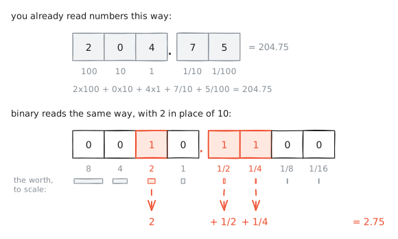
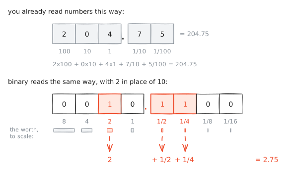
Read 0010.1100 with those place values: the 1s sit on 2, on a half and on a quarter, and 2 + 0.5 + 0.25 = 2.75. That is all a string of bits with a dot in it can mean, and you can now read any of them.
One question hides here, and it decides half of this page: which fractions can these places write exactly? The places are halves, quarters, eighths. Any finite sum of them is a fraction whose denominator is a power of 2: 1/2, 3/4, 5/8. Those end cleanly. Now take 1/3, 1/5 or 1/10. Their denominators carry a 3 or a 5. No finite sum of halves, quarters and eighths equals them. Watch both cases run: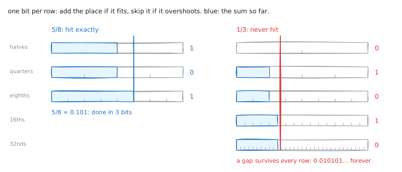
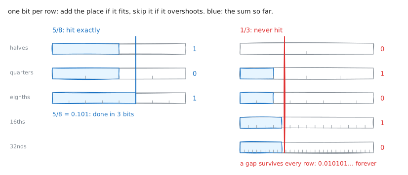
Decimal plays the same game with different equipment. Base 10 is 2 x 5, so it digests 2s and 5s. Base 2 digests only 2s: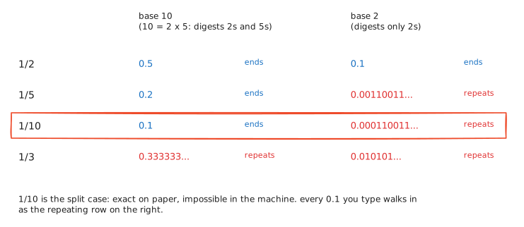
Now a first attempt that fails. Take 1 byte, which is 8 bits, and fix the dot in the middle: 4 bits for the whole part, 4 for the fraction: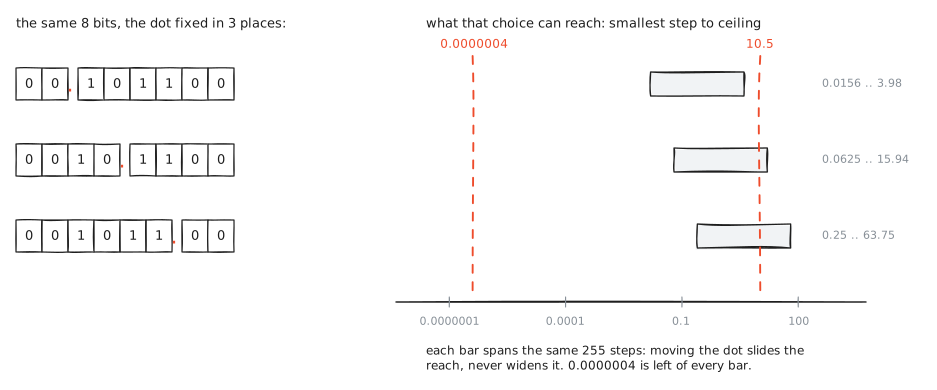
This is called fixed point, and the drawing shows its problem: the dot's position decides the largest value and the smallest step at the same time, and no single position makes both good. The repair is in the name of this page. Let the dot move, and store where it went.
Where should the machine write down "where the dot went"? You already know the answer, because you already do this on paper. To write a very small or a very large number, you split it into its digits and its size: 0.00000037 becomes 3.7 x 10^-7. The 3.7 says what the digits are; the 10^-7 says how big the number is. 2 separate jobs, written separately: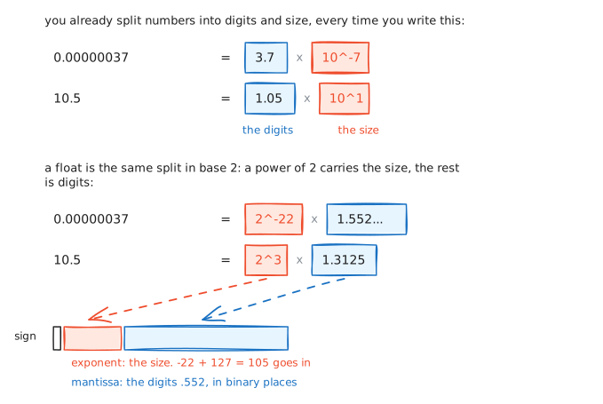
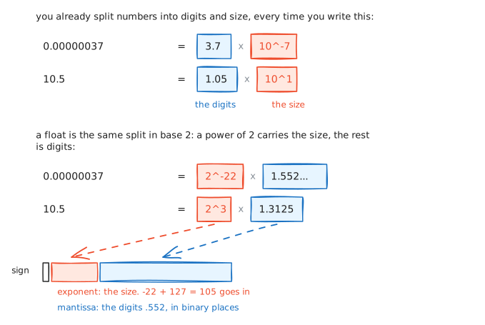
A float makes exactly this split, in base 2. Any positive number is some power of 2 times a number between 1 and 2: 10.5 is 1.3125 x 2^3 (check it: 2^3 = 8, and 1.3125 x 8 = 10.5), and 0.00000037 is about 1.552 x 2^-22. The power of 2 goes into one field, named the exponent. The 1.something goes into the other field, named the mantissa. The 2 words are only names for the 2 halves of the split: the exponent is the number's size, the mantissa is its digits.
What does each field buy on the number line? Draw them [2]: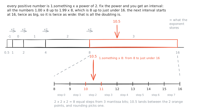
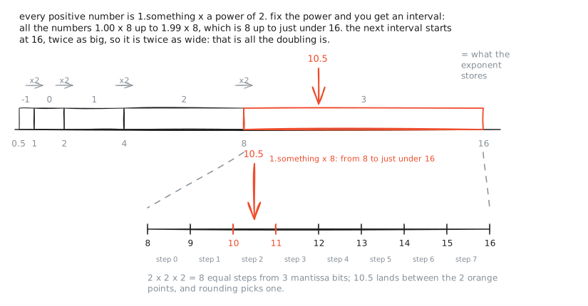
Where do the intervals come from? From the split itself. Fix the power at 8. The digits part runs from 1.00 to 1.99. So the values run from 8 to just under 16: every number with power 8 lives between 8 and 16. Fix the power at 16 and you fill 16 to 32. That stretch starts twice as high, so it is twice as wide. That is all the doubling is. And the powers go both ways. The power -1 gives the interval [1/2, 1). The power -2 gives [1/4, 1/2). Each of those is half as wide as the next. So the intervals climb away from 1 in both directions: growing above it, shrinking below it, until the exponent runs out of values. The leftmost box in the drawing, [0.5, 1), is the first of the shrinking ones. Choosing the exponent is choosing the interval. 8 exponent bits count 2^8 = 256 intervals, and because every interval doubles, 256 of them span an enormous distance: that is how 8 bits reach from 1e-38 to 3e38. The mantissa then cuts the chosen interval into equal steps: 3 bits make 2 x 2 x 2 = 8 steps, binary32's 23 bits make 8,388,608. And the growing step we asked for at the start falls out by itself: [4, 8) is twice as wide as [2, 4), both are cut into the same number of steps, so every step in [4, 8) is twice as long. Small numbers get fine steps, large numbers get coarse ones, with nobody managing it.
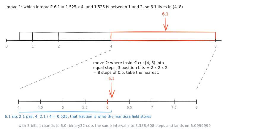
Now store one number end to end. Move 1: pick the interval. 6.1 = 1.525 x 4, and 1.525 is between 1 and 2, so the interval is [4, 8). Move 2: say where inside. 6.1 sits 2.1 past 4, and 2.1 / 4 = 0.525. That fraction, 0.525, is what the mantissa holds: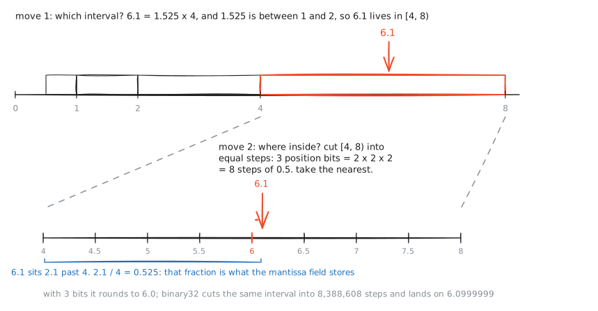
In a real 32-bit float the split gets 1 bit for the sign, 8 for the exponent, 23 for the mantissa. Here is 6.1, every field decoded: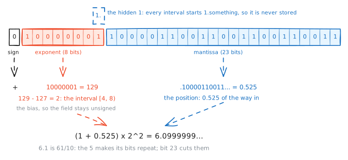
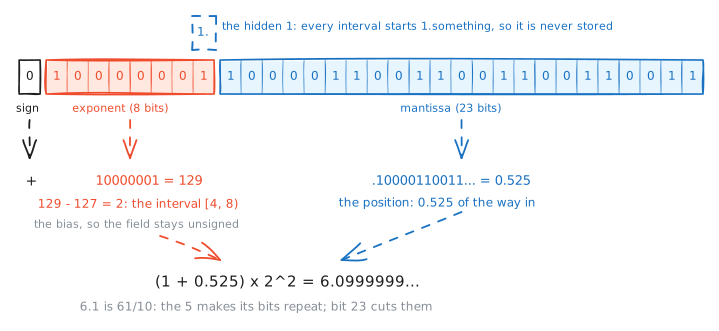
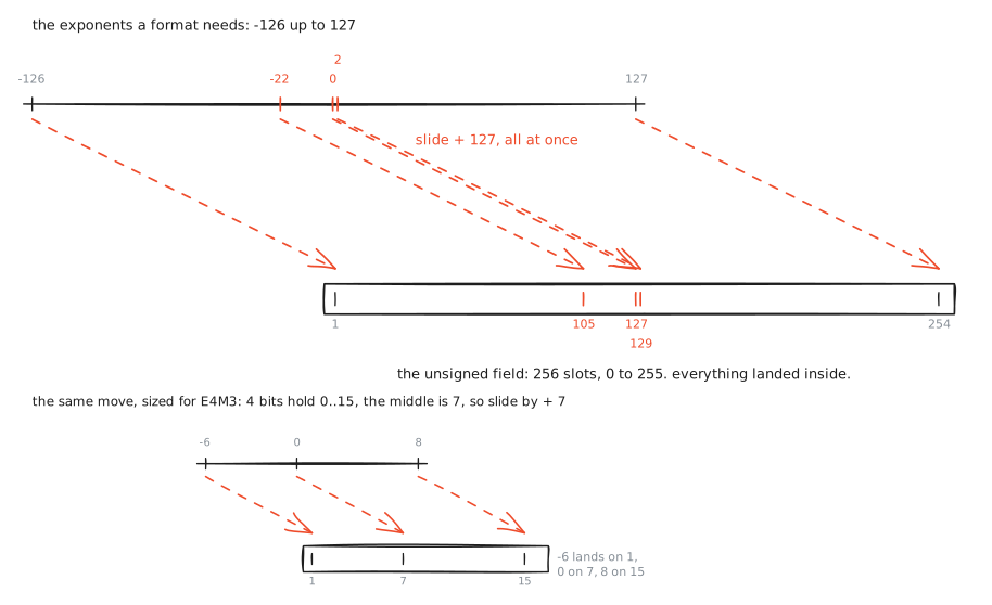
Two details in that card deserve their own sentences, because every format on this page inherits both. First, the decode row says "1 + 0.525", but the mantissa field only stored the .525. The leading 1 costs nothing: every number in a power-of-two interval is 1.something times a power of two, so the format does not store the 1 and gets 24 bits of position for the price of 23. (The subnormals, coming 2 sections from now, are 0.something and are the one exception.) Second, the bias. Here is the problem it solves. The exponent field is a box of 256 slots, numbered 0 to 255. Slot numbers cannot be negative. But the exponents we need to store run from -126 to 127: tiny numbers need negative ones. So the numbers we have do not fit the labels the box has. The fix is one move: slide every exponent up by the same constant, 127, picked because it is the middle of 0 to 255. After the slide, -126 sits in slot 1, -22 sits in slot 105, 0 sits in slot 127, 2 sits in slot 129, and 127 sits in slot 254. Nothing is reordered and nothing is lost; the whole line moved as one piece: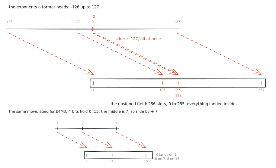
The stored slot number is the exponent plus the bias. So the two directions you saw earlier are just the slide and its undo: storing adds 127 (the -22 above went in as -22 + 127 = 105), and reading subtracts 127 (this card's 129 means 129 - 127 = 2). (Slots 0 and 255 are kept back; they build the edge cases 2 sections ahead.)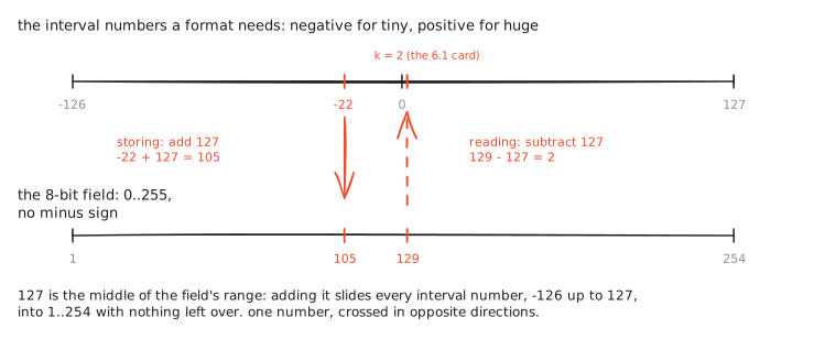
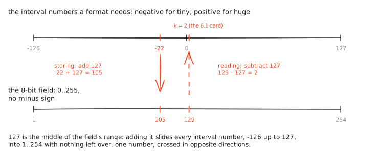
The rule behind 127 works in every format: the bias is the middle of what the exponent field can hold. 8 bits hold 0 to 255; the middle is 127. A 4-bit exponent field holds 0 to 15; the middle is 7, and you will meet that 7 on the next drawing.
The unsigned choice has a quiet payoff. A bigger float always carries a bigger bit pattern, so a chip can compare 2 floats with the integer circuits it already owns [3].
One practical question: when does the machine do all this splitting? Mostly never at run time. The 6.1 in your source is text, and the compiler turns it into these 32 bits once, before the program runs. The 2.1 / 4 in our story needs no divider either: 4 is a power of 2, so dividing by it only moves the dot 2 places. After an add or a multiply, the hardware slides the result's dot until a single 1 stands in front, counts the slide into the exponent, and keeps the digits as the mantissa. Slides and counts: the format's own bookkeeping never divides.
Notice what the last decode row admits: the machine does not store 6.1. It cannot. 6.1 is 61/10, and the 10 carries a 5. The fractions figure showed what a 5 does in base 2: the bits repeat forever. The mantissa keeps 23 of them and cuts the rest. What remains decodes to 6.0999999..., the nearest float32. The gap is the rounding error. The sections ahead measure that gap and follow its consequences. This layout, the bias and the field widths, was standardized in 1985 as IEEE 754 [3], and it is the format your float32 tensors use today, unchanged.
The map
You cannot draw all 4,294,967,296 points of float32. But the same design at 8 bits has only 2^8 = 256 patterns, and its entire positive half fits in one picture. The 8-bit format is called E4M3, and it is not a toy: it is the FP8 on your GPU's spec sheet, the format H100 tensor cores multiply in. The name is just its recipe: E4 means 4 exponent bits, M3 means 3 mantissa bits. Every format name on this page reads the same way. This is the most important drawing on this page, because every format you will ever meet is this drawing with different counts: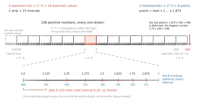
p2_e4m3_map.py the proof, ready to read or run
download and run it# every fp8 e4m3 value, decoded from its 8 bits by hand, then
# checked bit for bit against torch.float8_e4m3fn. 256 patterns is
# the entire format, and the decoder fits in a few lines.
import torch
def decode_e4m3(byte):
s = (byte >> 7) & 1 # 1 sign bit
e = (byte >> 3) & 0xF # 4 exponent bits
m = byte & 0x7 # 3 mantissa bits
if e == 0xF and m == 0x7:
return float("nan") # the one nan pattern per sign
if e == 0: # subnormal: no hidden 1
return (-1)**s * 2**(1 - 7) * (m / 8)
return (-1)**s * 2**(e - 7) * (1 + m / 8) # 7 is the bias
agree, values = 0, []
for byte in range(256):
mine = decode_e4m3(byte)
ref = torch.tensor([byte], dtype=torch.uint8).view(torch.float8_e4m3fn).float().item()
ok = (mine != mine and ref != ref) or mine == ref # nan == nan is false
agree += ok
if not ok:
print(f"DISAGREE byte {byte:08b}: mine {mine}, torch {ref}")
values.append(mine)
print(f"{agree}/256 bit patterns agree with torch.float8_e4m3fn")
finite = sorted(v for v in values if v == v)
pos = [v for v in finite if v > 0]
print(f"largest value : {max(finite)}")
print(f"smallest positive : {min(pos)}")
print(f"positive values : {len(pos)}")
print(f"step just above 1.0 : {min(v for v in pos if v > 1.0) - 1.0}")
print(f"step just below 448 : {448 - max(v for v in pos if v < 448)}")
# the run prints:
#
# 256/256 bit patterns agree with torch.float8_e4m3fn
# largest value : 448.0
# smallest positive : 0.001953125
# positive values : 126
# step just above 1.0 : 0.125
# step just below 448 : 32.0
#
# every number the map drew is here: 126 positive values because 2
# of the 128 positive patterns went to zero and nan, the ceiling at
# 448, the smallest positive at 2^-9 = 0.001953125, and the step
# growing from 0.125 near 1.0 to 32 near the top.
Read the map slowly; every later section builds on it. Start with one count. After the sign bit, E4M3 has 7 bits left. 7 bits make 2^7 = 128 patterns. One pattern is the number 0. One pattern is NaN. 128 - 2 = 126. That is the whole story of "126 positive numbers": every pattern is drawn except those 2.
Now place the points. The 4 exponent bits pick from 2^4 = 16 exponent values. The lowest one is the dashed strip at the far left; its points work differently, and the next section explains them. The other 15 are the 15 intervals you see. Which intervals are they? Read them off with the bias, exactly as in binary32, only smaller. E4M3's exponent field has 4 bits, holding 0 to 15, so its bias is the middle: 7. Stored values 1 to 15, minus 7, give the true powers -6 up to 8. So the leftmost interval is [2^-6, 2^-5), which is [0.0156, 0.0312), and the rightmost is [2^8, 2^9), which starts at 256. 6 intervals sit below 1, holding the tiny numbers; 9 sit at 1 and above, holding the big ones. The drawing writes the power under each boundary label. Inside any interval, the 3 mantissa bits place the 8 points, and they are always the same 8: the interval's start times 1, times 1.125, times 1.25, and so on up to times 1.875. Look at the zoom: for the interval [1, 2) that is exactly 1.0, 1.125, ... 1.875.
The 2 spent patterns are the 2 holes you can see. The zero pattern would have been the first point of the dashed strip, so the strip holds 7 points instead of 8. The NaN pattern is the last point of the top interval. That interval starts at 2^8 = 256, so its last point would have been 1.875 x 256 = 480; that pattern means NaN instead, and the drawing marks it red. The biggest real number is the point before it: 1.75 x 256 = 448. Check the count region by region: 7 in the strip, 8 in each of 14 intervals, 7 in the top one. 7 + 112 + 7 = 126. It matches.
Next, the idea this whole page stands on. Ask first: what should a good format promise you? Not a small miss. A small miss compared to your number. Missing by 0.5 when your number is 1.5 ruins it; missing by 0.5 when your number is 12,000 changes nothing you care about. So the fair way to judge a miss is as a share: the miss divided by the number it happened to. The next drawing judges 4 cases that way, and each share is drawn as a red fill so you can see it instead of computing it: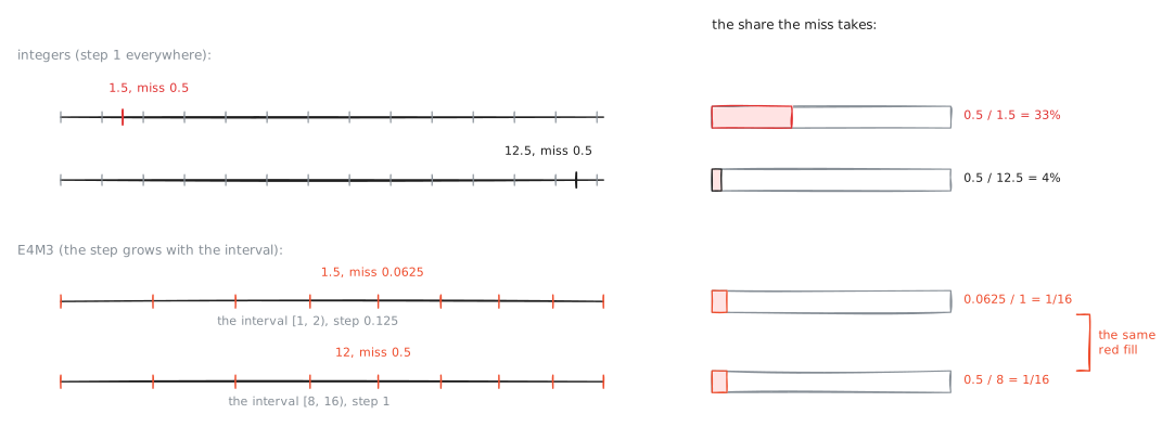
Read the 2 orange bars in the drawing: identical. Here is why, in one chain. An interval runs from its start to twice its start, so its width equals its start. 8 steps cut that width, so 1 step is the start divided by 8, and the worst miss, half a step, is the start divided by 16. Take the share: divide by the start, and the start cancels. 1/16, at every size. Now the 2 words this subject uses. Absolute error is the size of the miss; it doubles from interval to interval. Relative error is the share; a float pins it at the same value everywhere. Every float format works this way.
The local step also has a proper name, and you will meet it in every numerics discussion: the ulp, the unit in the last place [4]. "The ulp at x" means the step between neighboring points where x lives. E4M3's ulp at 1.0 is 0.125; its ulp at 300 is 32. One number is enough to know a format's whole precision: the ulp at 1.0. Every other interval's step is that same number, doubled or halved some number of times. So if you know the step in [1, 2), you know the step everywhere. The field guide ahead prints it on every card, as "step at 1.0".
The proof under the map is 15 lines of Python that decode all 256 bit patterns from first principles, and torch agrees with every single one. The largest value is 448. The smallest positive value is 0.001953125. Divide them: 448 / 0.001953125 = 229,376, about 2^17.8. Read the exponent as a count of doublings: start at the bottom, double about 18 times, and you reach the top. That count is the format's whole reach. Now compare it with the second drawing: one tensor's gradients needed 21 doublings. The whole format is narrower than one tensor's spread, and that gap runs the entire training half of this page.
The edges of the map
Four places on the map need special handling, and every format must decide all four.
Zero. The position field always means "1.something", so no pattern naturally means zero. The all-zeros pattern is simply assigned the value zero, as a special case. The sign bit still exists, so there is a +0 and a -0, and they compare equal.
The ramp. Just above zero there is trouble. Every normal point is 1.something x a power of 2. The exponent has a lowest power, so there is a smallest normal point. In E4M3 the lowest normal exponent value is 1 and the bias is 7, so the lowest power is 1 - 7 = -6, and the smallest normal point is 1.0 x 2^-6 = 0.015625. Below it, a naive format has nothing until 0. A cliff. The fix: in the lowest interval only, drop the hidden 1. Read the mantissa as 0.something instead of 1.something. Walk through what that gives. The pattern 000 reads 0.000 x 2^-6 = 0: zero itself. The pattern 001 reads 0.001 x 2^-6, which is 1/8 x 0.0156 = 0.00195. The pattern 010 gives 0.0039. And so on up to 111, which gives 0.0137. 7 evenly spaced points now fill the gap between 0 and 0.0156. These points are the subnormals. They turn the cliff into a ramp: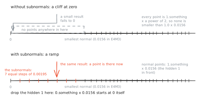
Infinity. When a result overflows the ceiling, float32 returns a dedicated pattern called inf, which then behaves lawfully: anything finite divided by inf is 0, and inf - inf is the next special value. E4M3 made a harder choice: it has no infinity at all. Those patterns were used for one more doubling of range, and overflow stops at 448 instead. Keep that choice in mind; it is the first sign of how little room 8 bits leave.
NaN. Not a Number is the pattern returned when no answer is defensible: 0/0, inf - inf, the square root of -1. It has one deliberately strange law: nan == nan is false, so x != x is the honest test for it. When your loss prints nan, this value is what you are looking at, and it arrived through an overflow or an undefined step somewhere upstream. We will catch it in the act in a few sections.
The field guide
The formats in this guide carry nearly all of the world's floating-point arithmetic, and you now own every idea needed to read them. Each gets the same treatment: its card, the bit counts and the numbers that follow from them; its map, where its points land; where it came from; where it runs today; and how it fails. One promise about the cards: none of their numbers is new information. Give the 2 bit counts, E and M, and every row follows by rules you already have. The bias is the middle of the E-bit range. The lowest and highest powers come from sliding the stored range back, so the ceiling and the floors follow. The step at 1.0 is 1 divided by 2^M. The digits count follows from the step. The brackets on each card point each row at the field that sets it, and the proof computes every row from E and M and checks it against torch's own tables (proof runs the check). The guide covers the 4 wide formats, the ones that stand alone. The 8-, 6- and 4-bit formats enter later, each at the exact place in the training story that needs it, and a closing sheet gathers the whole family on one drawing.
p16_wide_formats.py the proof, ready to read or run
download and run it# the field guide's numbers, derived by hand from each format's 2
# bit counts (E exponent bits, M mantissa bits), then checked
# against torch. nothing on the cards is typed from memory:
#
# bias = 2^(E-1) - 1
# ceiling = (2 - 2^-M) * 2^bias
# floor = 2^(1 - bias) smallest normal
# ramp floor = 2^(1 - bias - M) smallest subnormal
# step at 1 = 2^-M the ulp of 1.0; finfo calls it eps
# intervals = 2^E - 2 power-of-2 intervals
# points each = 2^M
#
# also prints the torch defaults the float32 section quotes.
import math
import torch
FORMATS = [
("float64", 11, 52, torch.float64, torch.int64),
("float32", 8, 23, torch.float32, torch.int32),
("float16", 5, 10, torch.float16, torch.int16),
("bfloat16", 8, 7, torch.bfloat16, torch.int16),
]
for name, E, M, dt, it in FORMATS:
bias = 2 ** (E - 1) - 1
ceiling = (2 - 2.0 ** -M) * 2.0 ** bias
floor = 2.0 ** (1 - bias)
ramp_floor = 2.0 ** (1 - bias - M)
step_at_1 = 2.0 ** -M
intervals = 2 ** E - 2
digits = (M + 1) * math.log10(2)
fi = torch.finfo(dt)
# smallest subnormal: the bit pattern 0...01 viewed as this dtype
sub = torch.tensor([1], dtype=it).view(dt).double().item()
assert ceiling == fi.max, (name, ceiling, fi.max)
assert floor == fi.tiny, (name, floor, fi.tiny)
assert step_at_1 == fi.eps, (name, step_at_1, fi.eps)
assert ramp_floor == sub, (name, ramp_floor, sub)
print(f"{name:9s} E={E:2d} M={M:2d} bias {bias:4d} "
f"ceiling {ceiling:.4g}")
print(f" floor {floor:.4g} ramp floor {ramp_floor:.4g} "
f"step at 1 = {step_at_1:.4g}")
print(f" {intervals} intervals of {2**M:,} points; "
f"about {digits:.1f} decimal digits "
f"(torch.finfo agrees on all four numbers)")
# absorption never leaves; it only moves. float64's step at 1e16 is 2.
x = torch.tensor(1e16, dtype=torch.float64)
print(f"\nfloat64: (1e16 + 1) - 1e16 = {((x + 1) - x).item():g}"
f" (the step at 1e16 is 2; the 1 is below half of it)")
# the defaults the float32 section quotes, read from this install
print(f"\ntorch {torch.__version__} defaults:")
print(f" default dtype {torch.get_default_dtype()}")
print(f" float32_matmul_precision "
f"{torch.get_float32_matmul_precision()!r}")
print(f" backends.cuda.matmul.allow_tf32 "
f"{torch.backends.cuda.matmul.allow_tf32}")
print(f" backends.cudnn.allow_tf32 "
f"{torch.backends.cudnn.allow_tf32}")
print(f" autocast dtype on cpu "
f"{torch.get_autocast_dtype('cpu')}")
# the run prints (torch 2.11.0, cpu):
#
# float64 E=11 M=52 bias 1023 ceiling 1.798e+308
# floor 2.225e-308 ramp floor 4.941e-324 step at 1 = 2.22e-16
# 2046 intervals of 4,503,599,627,370,496 points; about 16.0 decimal digits (torch.finfo agrees on all four numbers)
# float32 E= 8 M=23 bias 127 ceiling 3.403e+38
# floor 1.175e-38 ramp floor 1.401e-45 step at 1 = 1.192e-07
# 254 intervals of 8,388,608 points; about 7.2 decimal digits (torch.finfo agrees on all four numbers)
# float16 E= 5 M=10 bias 15 ceiling 6.55e+04
# floor 6.104e-05 ramp floor 5.96e-08 step at 1 = 0.0009766
# 30 intervals of 1,024 points; about 3.3 decimal digits (torch.finfo agrees on all four numbers)
# bfloat16 E= 8 M= 7 bias 127 ceiling 3.39e+38
# floor 1.175e-38 ramp floor 9.184e-41 step at 1 = 0.007812
# 254 intervals of 128 points; about 2.4 decimal digits (torch.finfo agrees on all four numbers)
#
# float64: (1e16 + 1) - 1e16 = 0 (the step at 1e16 is 2; the 1 is below half of it)
#
# torch 2.11.0 defaults:
# default dtype torch.float32
# float32_matmul_precision 'highest'
# backends.cuda.matmul.allow_tf32 False
# backends.cudnn.allow_tf32 True
# autocast dtype on cpu torch.bfloat16
#
# 4 formats, 16 derived numbers, 16 asserts, zero disagreements
# with torch.finfo. the same 5 formulas that built the e4m3 map
# build every card in the field guide.
float64
Double binary32's byte count and you get the format the 1985 standard called double precision: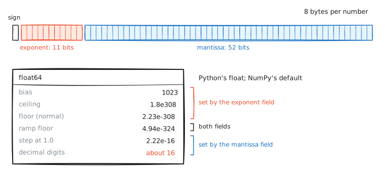
The bias is 1023, so the intervals run from 2.2e-308 up to 1.8e308: 2,046 of them, each holding 4,503,599,627,370,496 points. The ulp at 1.0 is 2.22e-16, which is about 16 decimal digits of position. A map that wide can only be drawn with breaks: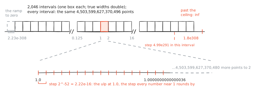
Where it came from: IEEE 754 began as the arithmetic William Kahan designed with Intel for the 8087, the floating-point coprocessor sold beside the 8086; the standards committee turned that chip's arithmetic into everyone's law [3][18]. float64 was its wide grade, sized so ordinary science could chain millions of operations and still trust the leading digits.
Where it runs today: everywhere you did not choose a dtype. A Python float is a float64. NumPy builds float64 arrays unless told otherwise. The rounding section ahead prints 0.1's stored digits; they are float64 digits.
Its proof: p16 derives the whole card from E and M and checks every row against torch.finfo. One extra line in it runs a vanishing add at this format's scale: in float64, (1e16 + 1) - 1e16 = 0. The ulp at 1e16 is 2, and the added 1 fell under half of it, so the sum rounded straight back (the failure section ahead names this absorption). 16 digits push the cliff out of sight; no digit count removes it.
How it fails in a training loop: float64 rarely gives training a wrong answer. Its problem is cost. 8 bytes per number is 2 times float32 and 4 times bfloat16, spent on digits training cannot use: the sections ahead show training running where the step at 1.0 is 0.0078, so digits 4 through 16 add nothing. On GPUs there is a second cost: most chips carry few float64 units, and NVIDIA's own throughput tables list float64 operations far below float32 on most of its hardware [19]. torch's default is float32, and float64 appears only when you ask (proof prints the default).
float32, and the format hiding inside it
binary32 you have already decoded by hand; the card collects its numbers: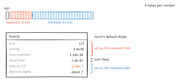
254 intervals from 1.2e-38 to 3.4e38, 8,388,608 points in each, about 7 digits: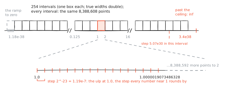
Where it came from: the same 1985 standard's single precision [3]. Where it runs today: it is the default dtype of torch; torch.tensor(1.0) is a float32 unless you say otherwise (proof prints the default from this install). Even when matmuls run narrow, the master weights of mixed-precision training stay float32 and the tensor cores accumulate in float32, so the training half of this page keeps this format at its center.
Now the format hiding inside it: TensorFloat-32. Since the A100, NVIDIA's tensor cores can take an ordinary float32 matmul, round each factor to 10 mantissa bits, multiply, and accumulate in full float32 [20]. The tensors going in and out are ordinary float32; only the multiply is narrow, reading 19 of the 32 bits (1 + 8 + 10). TF32 is that mode, not a storage type you can give a tensor. NVIDIA measured large speedups at matching accuracy on deep-learning workloads [20]; for code that needs all seven digits it is a silent cut, and that is why torch ships with matmul TF32 off since version 1.12 [21]. On this install, torch.backends.cuda.matmul.allow_tf32 is False, the cudnn convolution flag is True, and torch.set_float32_matmul_precision("high") is the one-line opt-in (proof prints all three). None of this can execute on the Apple machine this page is measured on; the flags are read here, the behavior is cited [20][21].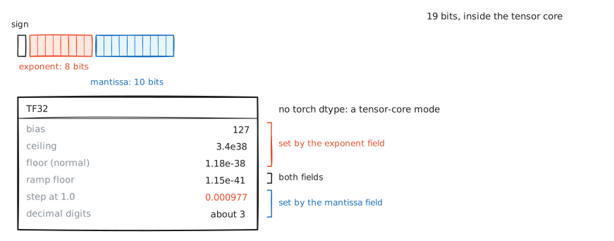
How it fails: you have watched it fail all page. The step of 8 at 1e8 is float32's. The 7 digits that turned a subtraction of near-equal inputs into a 19% error are float32's. In training, its failure is price: 4 bytes per number on the memory bus that a later section shows is the bottleneck.
float16
Cut 32 bits in half and something must go. There are two ways to choose, and the choice split the 16-bit world in two: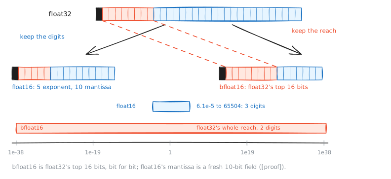
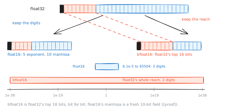
float16 is the left fork: keep digits, pay with reach.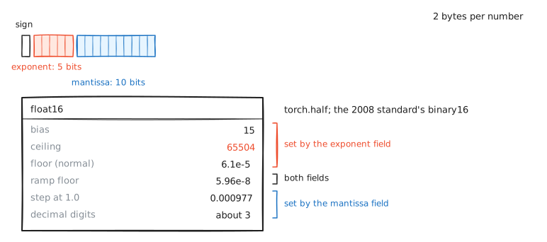
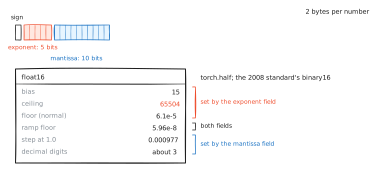
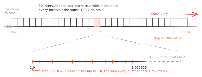
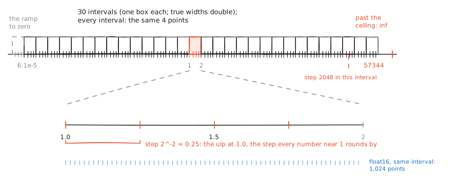
5 exponent bits give bias 15 and only 30 intervals, from 6.1e-5 to 65504. 10 mantissa bits give 1,024 points per interval and about 3 digits. 30 intervals fit in one drawing, so this is the one wide format whose map you can see whole: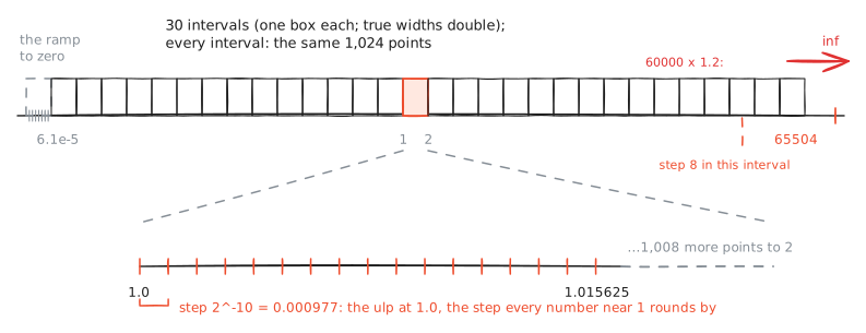
Where it came from: film and games, not a numerics committee. NVIDIA and Microsoft made half a type in the Cg shading language in 2002, and Industrial Light & Magic built its OpenEXR film format on the same 1+5+10 layout, in production from 2000 and released as open source in 2003 [22]. IEEE 754 adopted the layout as binary16 in its 2008 revision [3]. The film industry shipped the format years before the standard named it.
Where it runs today: graphics APIs and image pipelines still, inference engines, and mixed-precision training on hardware from before bfloat16 spread. In torch it is the half in .half().
Its proof and its failure are the same three numbers. The ceiling: 60000 times 1.2 is inf in float16 (proof). The digits: 1.001 stores as 1.000977. The floor: normal numbers end at 6.1e-5, and the small half of a gradient histogram lives below that, which is why the loss-scaling section exists. When float16 dies in a run, it dies at one of these three numbers.
p7_sixteen_bits.py the proof, ready to read or run
download and run it# the 16-bit fork, read straight from torch.finfo. nothing typed
# from memory.
#
# float16 spent its bits on precision (10 mantissa bits) and its
# ceiling sits at 65504. bfloat16 kept float32's 8 exponent bits,
# so it survives the same product, and pays with a step of 1/128
# at 1.0.
import torch
for dt in (torch.float32, torch.float16, torch.bfloat16):
fi = torch.finfo(dt)
print(f"{str(dt):16s} max {fi.max:>12.4g} tiny {fi.tiny:.3g} "
f"eps {fi.eps:.3g}")
# one multiplication that a training step could produce
x = torch.tensor(60000.0)
print(f"\n60000 * 1.2 in float16 : {(x.half() * 1.2).item()}")
print(f"60000 * 1.2 in bfloat16: {(x.bfloat16() * torch.tensor(1.2, dtype=torch.bfloat16)).item()}")
print(f"1.001 in float16 : {torch.tensor(1.001, dtype=torch.float16).item():.6f}")
print(f"1.001 in bfloat16 : {torch.tensor(1.001, dtype=torch.bfloat16).item():.6f}")
# the run prints:
#
# torch.float32 max 3.403e+38 tiny 1.18e-38 eps 1.19e-07
# torch.float16 max 6.55e+04 tiny 6.1e-05 eps 0.000977
# torch.bfloat16 max 3.39e+38 tiny 1.18e-38 eps 0.00781
#
# 60000 * 1.2 in float16 : inf
# 60000 * 1.2 in bfloat16: 72192.0
# 1.001 in float16 : 1.000977
# 1.001 in bfloat16 : 1.000000
#
# both sides of the trade in 4 lines: float16 overflows at 72000
# but resolves 1.001; bfloat16 reaches 72192 but rounds 1.001
# down to exactly 1, because its step at 1.0 is 0.0078 and the
# 0.001 is below half of it.
bfloat16
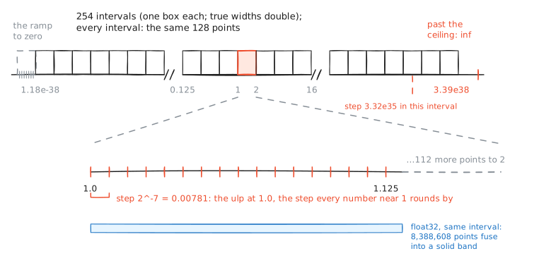
The right fork: keep reach, pay with digits. Google's brain float keeps all 8 of float32's exponent bits and 7 of mantissa: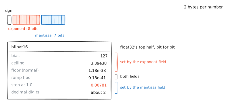
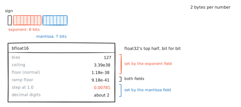
The reach is float32's (the ceiling prints 3.39e38 rather than 3.4e38 only because the coarser last step lands the top point lower), the intervals are the same 254 as float32's, and each holds 128 points: about 2 decimal digits.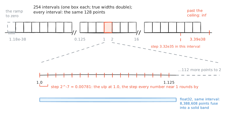
Where it came from: Google built it into the TPU's matrix units, which multiply in bfloat16 and accumulate in float32, and chose the layout so that range would never be the problem and conversion from float32 would be nearly free [23]. The name is Brain Floating Point, after the Google Brain team.
Nearly free is provable, and on this machine it is proven at the bit level: bfloat16 is float32's top half. Take any of the 65,536 possible bfloat16 bit patterns, cast it to float32, and the result is the same 16 bits with 16 zeros appended; proof checks all 65,536, bit for bit. The downward cast is the same move with rounding: keep the top 16 bits, round by the low 16. The proof checks torch's cast against that hand rule on 1,000,010 values (a million random ones plus the edge cases), and they agree on every one. Here is 1.7014 making the trip:
float32:  0 01111111 1011001 1100011101111010
bfloat16: 0 01111111 1011010   (the top half, rounded up by the rest)
stored:   1.703125
p17_bf16_truncation.py the proof, ready to read or run
# bfloat16 is the top 16 bits of float32, at the bit level. 2
# directions, both exhaustive where exhaustion is possible:
#
#   up:   every one of the 65,536 bfloat16 bit patterns, cast to
#         float32, must produce exactly (pattern << 16): the same
#         16 bits on top, 16 zeros appended below.
#   down: casting float32 to bfloat16 must equal keeping the top 16
#         bits and rounding by the low 16 (nearest, ties to even),
#         checked on a million random values plus the edge cases.
import torch

# up: bf16 -> fp32 is "append 16 zero bits", all 65,536 patterns
pats = torch.arange(65536, dtype=torch.int32).to(torch.int16)
as_bf16 = pats.view(torch.bfloat16)
up_bits = as_bf16.float().view(torch.int32)
want = pats.to(torch.int32) << 16
nan_mask = torch.isnan(as_bf16)
ok = (up_bits == want) | nan_mask
print(f"up-cast bit check: {ok.sum().item()} / 65536 patterns match "
      f"(pattern << 16)")
print(f"  of the 65536, {nan_mask.sum().item()} are NaN patterns, "
      f"checked separately:")
nan_ok = torch.isnan(as_bf16.float()[nan_mask]).all().item()
print(f"  every NaN pattern up-casts to a float32 NaN: {nan_ok}")
exact = (up_bits == want).sum().item()
print(f"  bit-exact including NaN payloads: {exact} / 65536")

# down: fp32 -> bf16 is "keep the top 16 bits, round by the rest"
def truncate_rne(f32):
    # the hand rule: add the rounding bias, then keep the top half.
    # bias = 0x7FFF plus bit 16, the classic nearest-even truncation
    u = f32.view(torch.int32)
    bias = 0x7FFF + ((u >> 16) & 1)
    out = ((u + bias) >> 16).to(torch.int16).view(torch.bfloat16)
    return torch.where(torch.isnan(f32), torch.nan, out.float())

torch.manual_seed(0)
x = torch.randn(1_000_000) * torch.logspace(-38, 38, 1_000_000)
edges = torch.tensor([0.0, -0.0, 1.0, 1.0078125, 65504.0, 3.4e38,
                      1e-40, float("inf"), float("-inf"), float("nan")])
x = torch.cat([x, edges])
ours = truncate_rne(x)
torchs = x.bfloat16().float()
agree = (ours == torchs) | (torch.isnan(ours) & torch.isnan(torchs))
print(f"\ndown-cast rule check: {agree.sum().item()} / {len(x)} "
      f"values agree with torch's cast")

# the picture, on one number
v = torch.tensor(1.7014, dtype=torch.float32)
u32 = v.view(torch.int32).item() & 0xFFFFFFFF
b16 = v.bfloat16().view(torch.int16).item() & 0xFFFF
print(f"\n1.7014 in float32 bits : {u32:032b}")
print(f"1.7014 in bfloat16 bits: {b16:016b} (the top half, rounded)")
print(f"bfloat16 value stored  : {v.bfloat16().item():.6f}")

# the run prints:
#
#   up-cast bit check: 65536 / 65536 patterns match (pattern << 16)
#     of the 65536, 254 are NaN patterns, checked separately:
#     every NaN pattern up-casts to a float32 NaN: True
#     bit-exact including NaN payloads: 65536 / 65536
#
#   down-cast rule check: 1000010 / 1000010 values agree with torch's cast
#
#   1.7014 in float32 bits : 00111111110110011100011101111010
#   1.7014 in bfloat16 bits: 0011111111011010 (the top half, rounded)
#   bfloat16 value stored  : 1.703125
#
# all 65,536 patterns up-cast bit-exactly, and a million and ten
# down-casts match the hand rule. "the top half of float32" is not
# a metaphor; it is the wiring.
Where it runs today: TPUs since their second generation [23], NVIDIA GPUs since the A100 [20], and this machine: torch's CPU autocast picks bfloat16 by default (proof prints it). In large-model training it is the usual compute half of the mixed-precision loop, with FP8 taking over the matmuls on the newest chips (the FP8 section returns to this).
How it fails: 2 digits. 1.001 stores as exactly 1.0 (proof). The step at 1.0 is 0.0078, so a healthy update of 0.001 sits under half a step and rounds away: the disaster that opens the training sections ahead, and the reason master weights exist. bfloat16 did not make training precise. It made training's failures the quiet, repairable kind, and the machinery that repairs them is most of the rest of this page.
The guide pauses here, because at 8 bits and below no format stands alone. Each narrow format arrives later on this page, at the moment the training story needs it, and a closing sheet gathers the whole family in one drawing. Next, with your formats on the table: what exactly happens in the space between two points, because every format above handles it the same way.
Rounding
Between any 2 neighboring points of the map lies everything the format cannot say. When a result lands there, one rule decides its fate: go to the nearer point. When it lands exactly halfway, there is a rule for the tie: go to the point whose last mantissa bit is 0. Half of the halfway cases end up rounding up and half down, so a long sum does not slowly lean one way. This pair of rules is round-to-nearest, ties-to-even, the default of every machine you will touch [3]: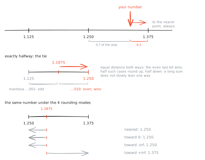
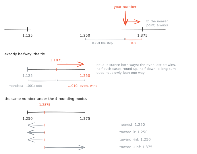
The worst this rule can do is move a value by half the local step: half an ulp. For float32 the ulp at 1.0 is 2 to the power -23, which is about 1.2e-7 (read e-7 as: move the decimal point 7 places left, so 0.00000012), and that number is called the machine epsilon (torch.finfo(torch.float32).eps prints it). So every operation lands within about 6e-8 of the true result, measured relative to the result's size. Both numbers read straight off the map: find the interval that starts at 1, take its step, halve it. The standard error analysis of floating point is this one bound, applied once per operation [4].
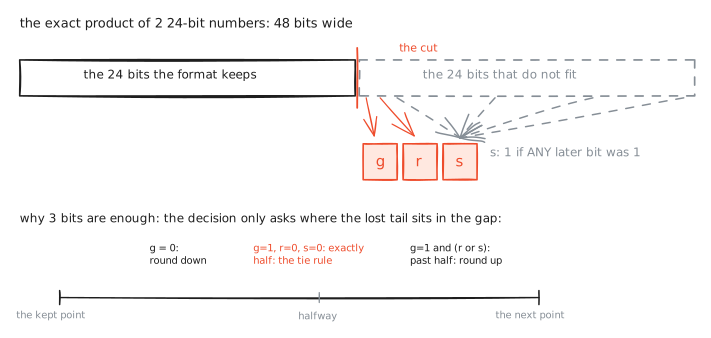
How can hardware apply the rule without computing every bit of the exact answer first? It keeps 3 extra bits, and that is all it ever needs: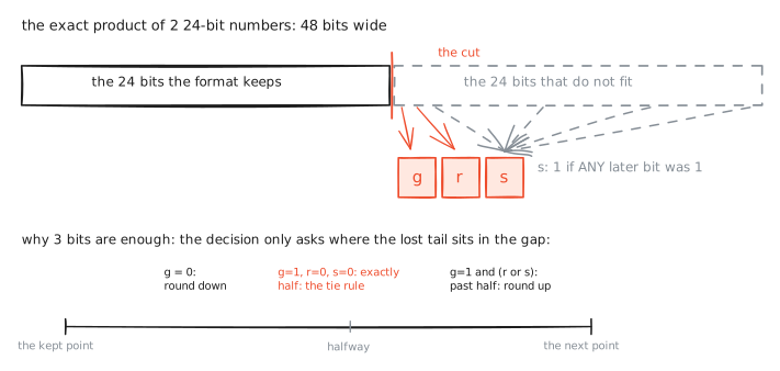
This explains the first code block at the top of the page, and you can check every step of it by hand. To write 0.1 in binary you double it, again and again, and each time the whole part of the result is the next bit. Why does doubling do that? Because in binary, doubling slides the dot 1 place, the same way multiplying by 10 slides the decimal dot. Whatever digit crosses the dot lands in front of it, and that digit is the next bit. 0.1 doubles to 0.2: the first bit is 0. Then 0.4, 0.8: two more 0s. Then 0.8 doubles to 1.6: the first 1, and the 0.6 carries on. 0.6 doubles to 1.2: another 1, and 0.2 carries on. But 0.2 is where the second step started. The process is in a loop, and the bits repeat forever: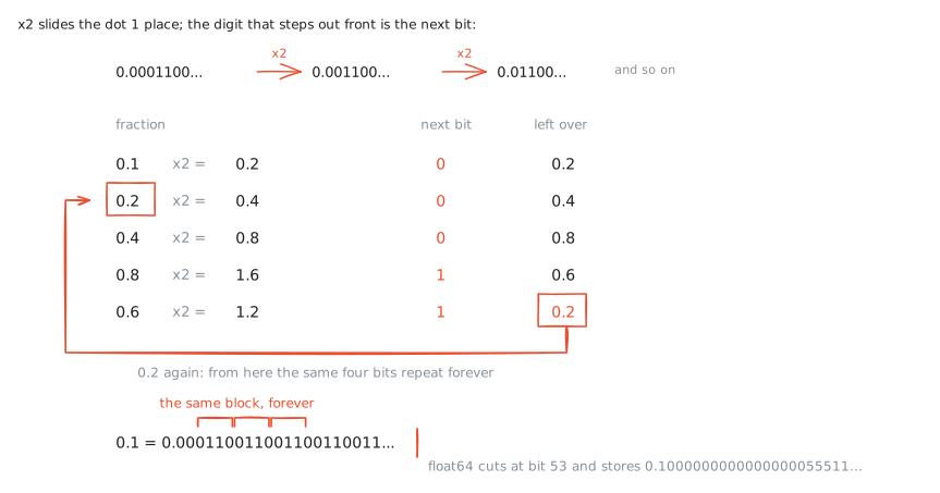
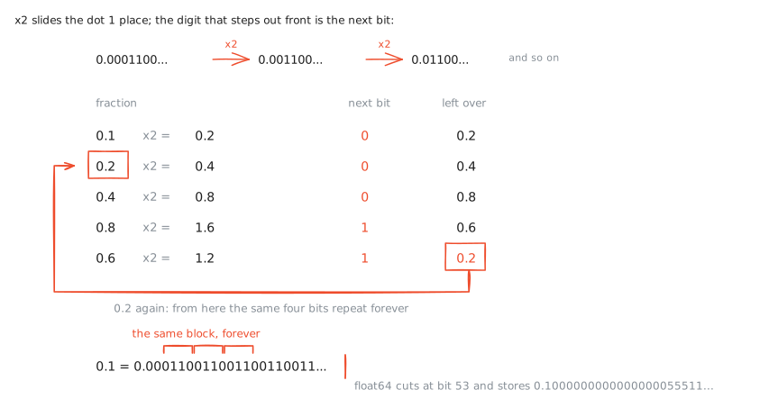
1/3 does the same thing in decimal, and for the same reason: the denominator has a prime factor the base does not. Ten is 2 times 5, so 0.1 is 1/(2 times 5), and base two has no 5. The format cuts the repetition at its mantissa width and stores the nearest representable number, which for float64 is exactly 0.1000000000000000055511151231257827... (proof prints every digit). The same happens to 0.2 and to 0.3, and the sum of the two stored numbers is not the stored number nearest 0.3. Nothing malfunctioned. 3 numbers you typed do not exist, and the printed digits show exactly which nearby numbers were stored instead.
p0_riddles.py the proof, ready to read or run
download and run it# the 2 riddles from the top of the page, run for real.
#
# riddle 1: 0.1 + 0.2 misses 0.3 because neither 0.1 nor 0.2 exists
# in binary. python stores the nearest float64 to each, and the sum
# of those 2 stand-ins is not the nearest float64 to 0.3.
#
# riddle 2: at 1e8, float32's numbers sit 8 apart. adding 1 asks for
# a move smaller than half that step, so the sum rounds straight
# back to where it started.
import torch
# 30 digits is enough to see it: the value you typed is already gone
# before any arithmetic happens
print(f"stored 0.1 = {0.1:.30f}")
print(f"stored 0.2 = {0.2:.30f}")
print(f"stored sum = {0.1 + 0.2:.30f}")
print(f"stored 0.3 = {0.3:.30f}")
print(f"0.1 + 0.2 == 0.3 : {0.1 + 0.2 == 0.3}")
print()
t = torch.tensor(1e8, dtype=torch.float32)
print(f"float32: 1e8 + 1 - 1e8 = {((t + 1) - t).item()}")
print(f"the local step at 1e8 = {torch.nextafter(t, torch.tensor(2e8)).item() - t.item()}")
# the run prints:
#
# stored 0.1 = 0.100000000000000005551115123126
# stored 0.2 = 0.200000000000000011102230246252
# stored sum = 0.300000000000000044408920985006
# stored 0.3 = 0.299999999999999988897769753748
# 0.1 + 0.2 == 0.3 : False
#
# float32: 1e8 + 1 - 1e8 = 0.0
# the local step at 1e8 = 8.0
#
# the stored sum and the stored 0.3 first differ in the 17th digit.
# each is the closest float the machine could pick; they just are
# not the same float. and at 1e8 the added 1 is below half of the
# local step of 8, so it rounds away to nothing.
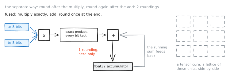
One more piece of standard equipment: the fused multiply-add, 1 instruction computing a times b plus c with a single rounding at the end instead of 2. The result is as if the product had been computed exactly and only the final sum were rounded, and on modern chips it costs about as much as 1 multiply [27]. The difference is not small print. Choose a = b = 1 + 2^-27 and c = -(1 + 2^-26): the separate path rounds the product first and returns exactly 0, while the fused path returns the true answer, 2^-54 (proof runs both on this machine). Every tensor core in the training half of this page is a lattice of these fused units, and the sums they accumulate stay in float32 even when the products arrive in 8 bits. Keep that sentence; it is why low-precision training is possible at all.
p21_fma_one_rounding.py the proof, ready to read or run
download and run it# the fused multiply-add really is one rounding instead of 2, and
# the difference is visible.
#
# choose a, b, c so the exact product a*b carries a tail the
# separate path must round away:
#
# a = b = 1 + 2^-27, so a*b = 1 + 2^-26 + 2^-54 exactly
# c = -(1 + 2^-26)
#
# the separate path rounds a*b to 1 + 2^-26 (the 2^-54 tail is
# under half an ulp), then adds c and returns exactly 0.0: it
# reports that a*b + c is zero when it is not. the fused path
# computes the exact product, adds c, rounds once, and returns the
# true answer, 2^-54. both answers are legal for the source line
# "a*b + c", which is why a compiler's fusion choice can change a
# program's bits.
import math
import torch
a = b = 1.0 + 2.0 ** -27
c = -(1.0 + 2.0 ** -26)
separate = a * b + c
if hasattr(math, "fma"):
fused = math.fma(a, b, c) # python 3.13+
how = "math.fma"
else:
import ctypes, ctypes.util
libm = ctypes.CDLL(ctypes.util.find_library("m"))
libm.fma.restype = ctypes.c_double
libm.fma.argtypes = [ctypes.c_double] * 3
fused = libm.fma(a, b, c) # the c library's fma
how = "libm fma"
print(f"a = b = 1 + 2^-27, c = -(1 + 2^-26)")
print(f"separate (a*b) + c : {separate}")
print(f"fused fma(a, b, c) : {fused} (via {how})")
print(f"true answer : {2.0 ** -54}")
assert separate == 0.0
assert fused == 2.0 ** -54
t = (torch.tensor(a, dtype=torch.float64) *
torch.tensor(b, dtype=torch.float64) +
torch.tensor(c, dtype=torch.float64)).item()
print(f"torch eager a*b+c : {t} (separate ops: also 0.0)")
print("\nthe separate path says the answer is exactly 0 when it is")
print("not; the fused path keeps it. both are legal readings of the")
print("same source line, which is why fusion decisions (a compiler")
print("flag, an inlined function, torch.compile) can change a")
print("program's last bits without anyone touching the math.")
# the run prints:
#
# a = b = 1 + 2^-27, c = -(1 + 2^-26)
# separate (a*b) + c : 0.0
# fused fma(a, b, c) : 5.551115123125783e-17 (via libm fma)
# true answer : 5.551115123125783e-17
# torch eager a*b+c : 0.0 (separate ops: also 0.0)
#
# 5.551115123125783e-17 is 2^-54 printed in decimal. the 2 asserts
# passed: the separate path really does return 0.0 and the fused
# path really does return the exact residue, on this machine, from
# the same source expression.
The unit itself is worth one look, because the training half of this page keeps returning to it: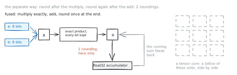
Where arithmetic goes wrong
Three rules of ordinary arithmetic stop holding once every result is rounded to a point, and all three cause real bugs.
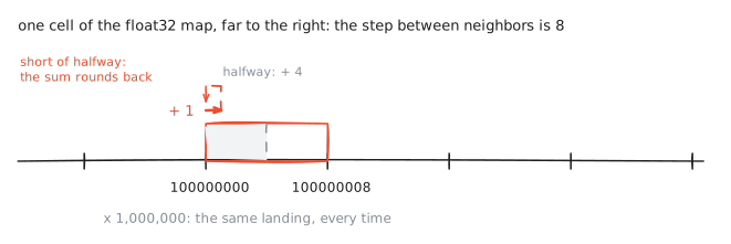
Absorption. At 100,000,000, which is 1e8, float32's step is 8, so adding 1 offers a move smaller than half the gap, and the sum rounds straight back (proof):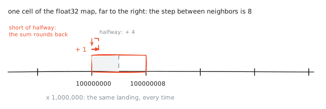
p4_absorb_cancel.py the proof, ready to read or run
download and run it# the 2 classic accidents, isolated.
#
# absorption: an addend below half the local step vanishes; one just
# past half the step rounds up to a full step.
#
# cancellation: subtracting 2 close numbers deletes their shared
# leading digits and promotes the inputs' rounding noise to the
# front of the result.
import torch
t = torch.tensor(1e8, dtype=torch.float32)
print(f"float32 step at 1e8 : {(torch.nextafter(t, t*2) - t).item()}")
print(f"1e8 + 1 : {(t + 1).item():.1f} (absorbed)")
print(f"1e8 + 5 : {(t + 5).item():.1f} (rounds up: past half the step)")
a = torch.tensor(1.0000001, dtype=torch.float32)
b = torch.tensor(1.0000000, dtype=torch.float32)
d = (a - b).item()
print(f"\n(1.0000001 - 1.0) in float32 = {d:.10e}")
print(f"true answer = 1.0000000e-07")
print(f"relative error = {abs(d - 1e-7)/1e-7:.1%}")
print("seven leading digits matched and left; only the rounding")
print("noise of the inputs remained.")
# the run prints:
#
# float32 step at 1e8 : 8.0
# 1e8 + 1 : 100000000.0 (absorbed)
# 1e8 + 5 : 100000008.0 (rounds up: past half the step)
#
# (1.0000001 - 1.0) in float32 = 1.1920928955e-07
# true answer = 1.0000000e-07
# relative error = 19.2%
# seven leading digits matched and left; only the rounding
# noise of the inputs remained.
#
# the 19.2% is not the subtraction's fault: 1.0000001 was stored
# with a tiny rounding error, invisible behind 8 total digits.
# the subtraction removed the 7 matching digits and left that
# error standing alone.
Cancellation. Subtract two nearly equal numbers and their shared front digits erase each other. Whatever rounding noise the inputs carried is suddenly the front of the answer: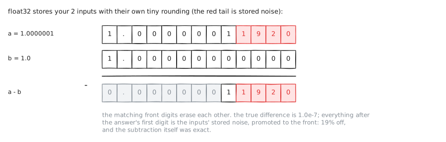
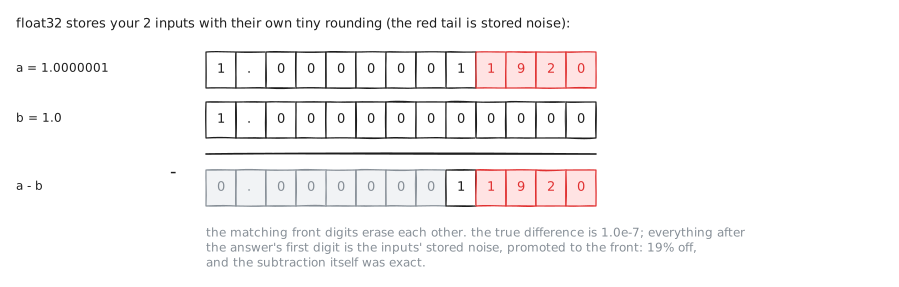
The proof above subtracts 1.0000001 from 1.0 in float32 and gets 1.19e-7 where the truth is 1.0e-7: a 19% error from one subtraction of two almost-exact inputs. The strange part: the subtraction itself commits no error at all. When 2 numbers are within a factor of 2 of each other, their difference is always exactly representable (Sterbenz's lemma [4]; proof checks it on this very case). Cancellation never creates error; it exposes the error the inputs already carried.
Order. Because every addition rounds, (a + b) + c and a + (b + c) are different numbers. The smallest possible example, drawn: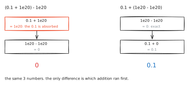
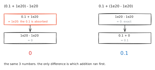
Sum 50,000 values forward and backward and the answers disagree (proof); a parallel machine that splits the same sum across cores picks yet another order, and another answer. torch's own .sum() adds pairwise in a tree, which is both faster and about 130 times closer to the true sum than a one-by-one loop (measured: 0.24 error against 0.0018), and compensated summation (Kahan's trick of carrying the rounding error in a second variable) closes most of the rest [4].
p5_sum_order.py the proof, ready to read or run
download and run it# addition order changes the answer.
#
# sum the same float32 values in 3 different orders and get 3
# different results; math.fsum on the float64 copies serves as the
# exact reference. torch's own .sum() reduces in a tree (pairwise),
# which is both faster and closer to the truth than a plain
# left-to-right fold.
import math, torch
torch.manual_seed(0)
x = (torch.randn(1_000_000) * 100).float()
# fold the values one by one, strictly in the given order, every
# intermediate rounded to float32. a python loop over a million
# tensors is slow, so run it on a 50,000-value slice; one order
# swap is enough to show the effect.
def fold(t):
s = torch.tensor(0.0, dtype=torch.float32)
for v in t.split(4096):
for u in v.tolist():
s = s + torch.tensor(u, dtype=torch.float32)
return s.item()
seq_fwd = fold(x[:50_000])
seq_rev = fold(x[:50_000].flip(0))
tsum = x[:50_000].sum().item() # torch's pairwise-style reduction
truth50 = math.fsum(x[:50_000].double().tolist())
print(f"ground truth (fsum) : {truth50:.6f}")
print(f"sequential, forward : {seq_fwd:.6f} err {seq_fwd-truth50:+.6f}")
print(f"sequential, reversed : {seq_rev:.6f} err {seq_rev-truth50:+.6f}")
print(f"torch .sum() (pairwise) : {tsum:.6f} err {tsum-truth50:+.6f}")
print(f"forward == reversed : {seq_fwd == seq_rev}")
# the run prints (seeded, so the same everywhere):
#
# ground truth (fsum) : -35811.271616
# sequential, forward : -35811.515625 err -0.244009
# sequential, reversed : -35811.398438 err -0.126821
# torch .sum() (pairwise) : -35811.273438 err -0.001821
# forward == reversed : False
#
# same 50,000 numbers, and reversing them moves the sum by 0.12.
# the tree reduction is 100x closer to the truth than either
# straight fold, because its partial sums stay similar in size and
# absorb less.
One more fact turns this whole section from a list of failures into a toolbox: the rounding error is catchable, exactly. When s = a + b rounds, the missing sliver is itself a number the format can hold, and 3 operations hand it back whole: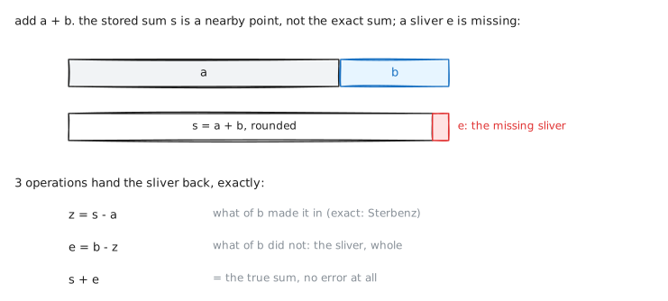
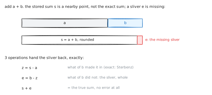
Run it on this page's opening example and the 3 operations hand back the exact rounding error of 0.1 + 0.2 (proof checks it against exact rational arithmetic). A fused multiply-add does the same for a product in 1 instruction. Kahan's compensated sum is this trick run in a loop, and the double-word arithmetic that stretches precision in software is this trick kept instead of thrown away [4].
p22_exact_error.py the proof, ready to read or run
download and run it# the rounding error is catchable, exactly. 3 facts, each checked
# against exact rational arithmetic (fractions.Fraction):
#
# 1. fast2sum: for |a| >= |b|, 3 operations recover the rounding
# error of a + b perfectly: s = a+b; z = s-a; e = b-z. then
# s + e equals the true sum of the stored a and b, exactly.
# run on the page's opening example, 0.1 + 0.2.
# 2. sterbenz: when x and y are within a factor of 2 of each other,
# x - y is computed exactly: cancellation commits no error of
# its own; it only exposes error the inputs carried.
# 3. 2multfma: one fused multiply-add recovers a product's whole
# rounding error: e = fma(a, b, -a*b).
from fractions import Fraction as F
import ctypes, ctypes.util
# fact 1: fast2sum on 0.1 + 0.2
a, b = 0.2, 0.1
s = a + b
z = s - a
e = b - z
print(f"s = a + b = {s!r}")
print(f"e = (b - (s - a)) = {e!r}")
assert F(a) + F(b) == F(s) + F(e) # exact rational check
print("checked: stored 0.2 + stored 0.1 == s + e, exactly.")
print("the 3 float operations caught the rounding error whole.\n")
# fact 2: sterbenz, close subtraction is exact
x, y = 1.0000001, 1.0
d = x - y
assert F(x) - F(y) == F(d)
print(f"x - y = {d!r}")
print("checked: equals the exact difference of the stored inputs.")
print("the 19% error of the cancellation section was already in")
print("the inputs; the subtraction added nothing.\n")
# fact 3: 2multfma, a product's error in one instruction
libm = ctypes.CDLL(ctypes.util.find_library("m"))
libm.fma.restype = ctypes.c_double
libm.fma.argtypes = [ctypes.c_double] * 3
u = v = 1.0 + 2.0 ** -27
p = u * v
e2 = libm.fma(u, v, -p)
assert F(u) * F(v) == F(p) + F(e2)
print(f"p = u * v = {p!r}")
print(f"e = fma(u,v,-p) = {e2!r}")
print("checked: stored u times stored v == p + e, exactly.")
print("\nKahan's compensated sum is fact 1 run in a loop; the")
print("double-word arithmetic that stretches precision in software")
print("is facts 1 and 3 kept instead of thrown away.")
# the run prints:
#
# s = a + b = 0.30000000000000004
# e = (b - (s - a)) = -2.7755575615628914e-17
# checked: stored 0.2 + stored 0.1 == s + e, exactly.
# the 3 float operations caught the rounding error whole.
#
# x - y = 1.0000000005838672e-07
# checked: equals the exact difference of the stored inputs.
# the 19% error of the cancellation section was already in
# the inputs; the subtraction added nothing.
#
# p = u * v = 1.0000000149011612
# e = fma(u,v,-p) = 5.551115123125783e-17
# checked: stored u times stored v == p + e, exactly.
#
# every assert compares floats against fractions.Fraction, which
# is exact rational arithmetic with no rounding at all. all 3
# held: the machine's own operations can hand back the error they
# just committed, to the last bit.
Keep the order fact in mind. It returns at the end of this page as the reason two identical training runs on two GPUs never match to the last bit.
The little epsilons, explained
Open any model's source code and small constants appear: an eps=1e-5 in the layer norm, an eps=1e-8 in Adam, a logits - logits.max() in every attention implementation. None of them is superstition; each one is a patch over a place where a formula's intermediate value leaves the map.
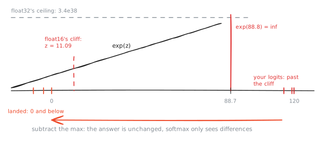
The largest number float32 can hold is about 3.4e38, and exp reaches it at 88.73 (measured below). Softmax, the function that turns a model's raw output scores, its logits, into probabilities, applies exp to every logit. Logits above 88.73 exist in every large model, so a naive softmax returns inf, then inf divided by inf, and your loss prints nan. The repair costs nothing: softmax only sees differences, so subtract the maximum first and the largest input becomes 0 (proof):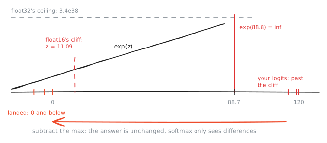
p6_stability.py the proof, ready to read or run
download and run it# the stability patterns.
#
# exp overflows just above 88.7 in float32 and just above 11.0 in
# float16, so a naive softmax dies on logits a model produces every
# day. subtracting the max before exp changes nothing mathematically
# (softmax is shift-invariant) and fixes it completely.
import torch
print(f"float32 exp cliff: exp(88.7)={torch.tensor(88.7).exp().item():.3e}, "
f"exp(88.8)={torch.tensor(88.8).exp().item()}")
h = torch.tensor([11.0, 11.1], dtype=torch.float16)
print(f"float16 exp cliff: exp(11.0)={h.exp()[0].item()}, exp(11.1)={h.exp()[1].item()}")
# logits of this size are ordinary in a large model
logits = torch.tensor([120.0, 119.0, 115.0])
naive = logits.exp() / logits.exp().sum()
stable = (logits - logits.max()).exp() / (logits - logits.max()).exp().sum()
print(f"naive softmax([120,119,115]) = {naive.tolist()}")
print(f"stable softmax([120,119,115]) = {[round(v,4) for v in stable.tolist()]}")
print(f"torch.softmax agrees with stable: "
f"{torch.allclose(torch.softmax(logits, 0), stable)}")
# logsumexp has the same illness and the same cure
print(f"naive log(sum(exp)) = {logits.exp().sum().log().item()}")
print(f"stable logsumexp = {torch.logsumexp(logits, 0).item():.4f}")
# the run prints:
#
# float32 exp cliff: exp(88.7)=3.326e+38, exp(88.8)=inf
# float16 exp cliff: exp(11.0)=59872.0, exp(11.1)=inf
# naive softmax([120,119,115]) = [nan, nan, nan]
# stable softmax([120,119,115]) = [0.7275, 0.2676, 0.0049]
# torch.softmax agrees with stable: True
# naive log(sum(exp)) = inf
# stable logsumexp = 120.3182
#
# 3 ordinary logits, and the naive path returns 3 nans: exp(120)
# overflows to inf, and inf / inf is nan. the shifted path never
# leaves float32's range, and torch.softmax is doing exactly this
# shift for you.
The same pattern explains the rest of the family, one line each. logsumexp slides by the max, for the same reason softmax does. log1p(x) and expm1(x) exist because near zero, 1 + x absorbs the x: the absorption figure again, happening at 1.0 instead of 1e8. The layer-norm epsilon keeps a near-zero variance from turning rsqrt into inf. Adam's epsilon guards its denominator the same way. And an attention mask uses a large negative number instead of -inf, so that after the slide it becomes a clean 0 instead of a nan. One picture, many patches: keep every in-between value where the points are.
Why smaller floats
The guide paused at 16 bits. Here is why the family keeps going down anyway.
Think about what training actually spends its time on. Mostly it moves numbers. Weights travel from memory to the arithmetic. Gradients travel back. Billions of numbers, every step. And the wire that carries them is slower than the multipliers that use them. Now halve the bits per number. The same wire carries twice the numbers. The same memory holds twice the model. The tensor cores, built for the narrower type, double their arithmetic too. One halving, three payoffs. Here is the wire, drawn to scale: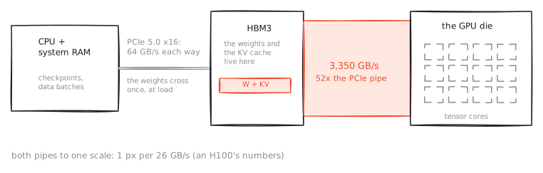
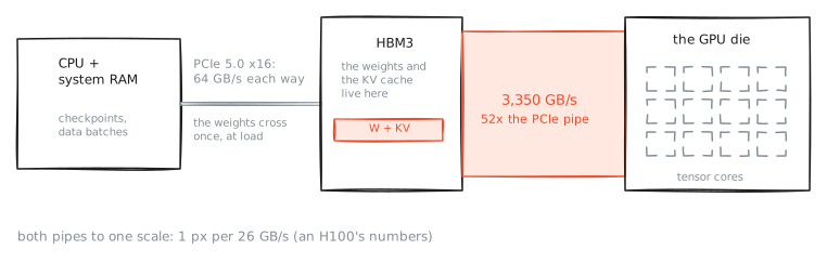
The only question is whether the surviving points still cover the numbers the network produces with small enough error. Networks tolerate rounding noise unusually well: they are trained on noisy batches and judged over many outputs, so the answer stays yes far below 32 bits if the format is chosen carefully. The fork figure already showed the first halving's two options, and training mostly picked bfloat16: reach first. The cost is a step of 0.0078 at 1.0, and the next section shows what that step does to learning.
The update that vanished
At 16 bits the map's steps are wide enough to stop training itself. A bfloat16 weight sitting at 1.0 has neighbors 0.0078 away. A healthy update of 0.001 is an arrow one eighth of that step: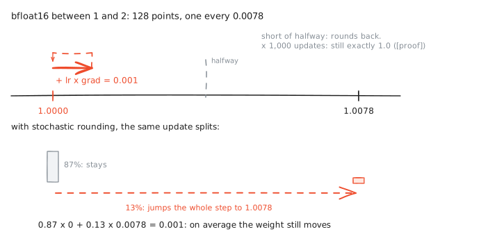
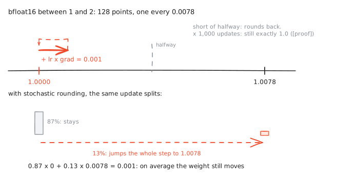
The proof runs it: 1,000 consecutive updates of 0.001 leave a bfloat16 weight at exactly 1.0 (proof). Not slowed. Stopped, silently, for that weight. This is why every mixed-precision recipe since 2017 keeps a float32 master copy of the weights [5]. The forward and backward passes run narrow. But the update lands in the float32 copy, where the local step is 65,536 times finer and 0.001 fits with room to spare. The other repair is stochastic rounding, which we will need again at 4 bits: round up with probability proportional to how far you got. In the same proof, the stochastically rounded weight reaches 2.0 alongside the master copy.
p8_lost_update.py the proof, ready to read or run
download and run it# the update that vanished.
#
# in bfloat16, a weight near 1.0 has a local step of 1/128, about
# 0.0078. an update smaller than half that step rounds away, and
# training silently stops for that weight. the float32 master copy
# is one fix; stochastic rounding is the other.
import torch
w = torch.tensor(1.0, dtype=torch.bfloat16)
u = 1e-3 # lr * grad, a normal size
print(f"bf16 next after 1.0 : {torch.nextafter(torch.tensor(1.0, dtype=torch.bfloat16), torch.tensor(2.0, dtype=torch.bfloat16)).item():.6f}")
print(f"w + {u} in bf16 : {(w + torch.tensor(u, dtype=torch.bfloat16)).item():.6f} (unchanged: {(w + torch.tensor(u, dtype=torch.bfloat16)) == w})")
# now 1000 such updates, 3 ways
steps = 1000
# way 1: accumulate in bfloat16 itself
wb = torch.tensor(1.0, dtype=torch.bfloat16)
for _ in range(steps):
wb = wb + torch.tensor(u, dtype=torch.bfloat16)
# way 2: keep a float32 master copy, the mixed-precision recipe
wm = torch.tensor(1.0, dtype=torch.float32)
for _ in range(steps):
wm = wm + u
# way 3: stochastic rounding, emulated. round up with probability
# equal to how far the true value sits between its 2 bf16 neighbors
g = torch.Generator().manual_seed(0)
ws = torch.tensor(1.0, dtype=torch.float32)
for _ in range(steps):
hi = torch.nextafter(ws.to(torch.bfloat16), torch.tensor(2.0, dtype=torch.bfloat16)).float()
lo = ws.to(torch.bfloat16).float()
x = ws + u
p = ((x - lo) / (hi - lo)).clamp(0, 1)
ws = hi if torch.rand((), generator=g) < p else lo
print(f"after {steps} updates of {u}:")
print(f" bf16 accumulate : {wb.item():.4f} (true answer 2.0)")
print(f" fp32 master : {wm.item():.4f}")
print(f" bf16 + stochastic : {ws.item():.4f}")
# the run prints:
#
# bf16 next after 1.0 : 1.007812
# w + 0.001 in bf16 : 1.000000 (unchanged: True)
# after 1000 updates of 0.001:
# bf16 accumulate : 1.0000 (true answer 2.0)
# fp32 master : 2.0000
# bf16 + stochastic : 2.0000
#
# 1000 updates that should have doubled the weight, and the pure
# bf16 path is still exactly 1.0: every single update rounded away.
# the master copy lands on 2.0, and so does stochastic rounding,
# because rounding up 1/8th of the time is worth exactly as much
# as adding the too-small update every time.
So the loop that trains every model you use runs like this: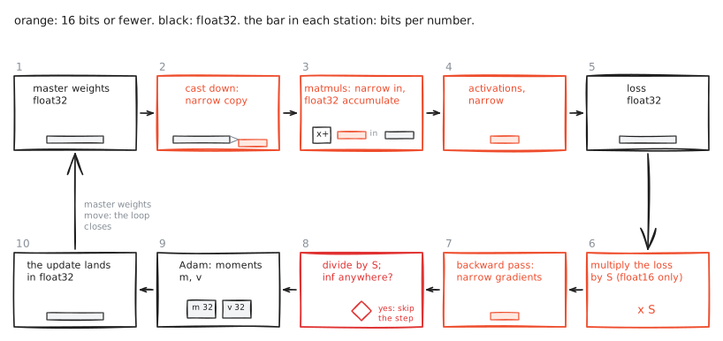
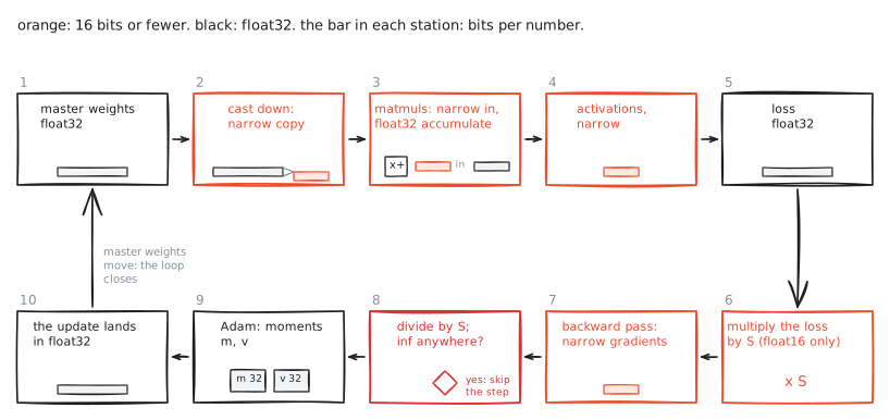
The products accumulate in float32 inside the tensor cores: that is the fused multiply-add from the rounding section doing its job. Precision goes exactly where the numbers need it and nowhere else. Stations 6 and 8, the S dial and the inf check, are the subject of the next section.
Loss scaling
One group of numbers still fails inside this loop. Gradients are the smallest numbers in training, and float16's floor is high: its subnormals end near 6e-8 and its normal range starts at 6e-5. The left tail of the gradient distribution simply falls below every point of the format: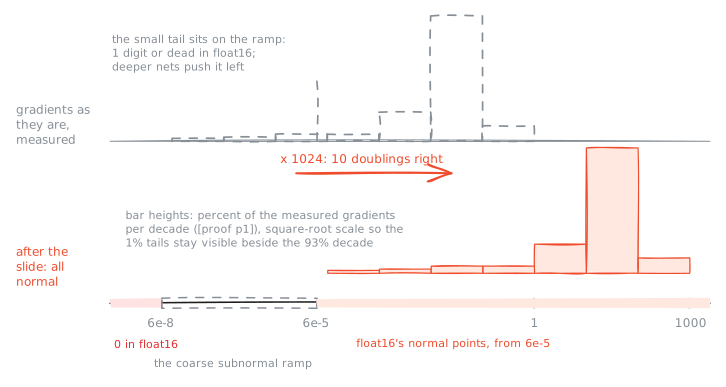
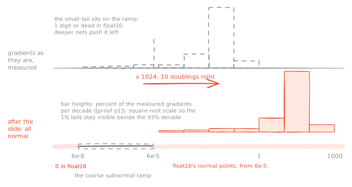
The rescue is one multiplication. Multiply the loss by a number S before the backward pass. Gradients are built from the loss by multiplications and additions, so every gradient comes out S times bigger, and the whole histogram slides right, into the band where float16 has points. Divide by S afterward. Nothing about the mathematics changed; the only difference is which gradients survived the trip. In practice S adjusts itself: see an overflow, halve S and skip that step; survive a stretch of clean steps, double it. That is the whole of GradScaler (proof measures the cast; on our toy net only 0.1% of gradients die, and the fraction grows with depth and training time, which is why the recipe exists [5]). bfloat16 mostly retired this machinery: it keeps float32's reach, so its normal floor sits at 1.2e-38 against float16's 6.1e-5, about 34 powers of 10 lower, and the scaler became optional.
p9_loss_scaling.py the proof, ready to read or run
download and run it# loss scaling, measured on real gradients.
#
# take float32 gradients from a small net, cast them to float16 as
# mixed precision must, and count the ones that flush to zero. then
# scale by 1024 first, cast, and unscale: the cast is where
# gradients die, and the scale is the rescue.
import torch, torch.nn as nn
torch.manual_seed(0)
net = nn.Sequential(nn.Linear(64, 256), nn.ReLU(),
nn.Linear(256, 256), nn.ReLU(), nn.Linear(256, 1))
X = torch.randn(2048, 64); y = X[:, :3].prod(1, keepdim=True)
loss = ((net(X) - y) ** 2).mean()
loss.backward()
g = torch.cat([p.grad.flatten() for p in net.parameters()])
nz = g[g != 0] # only true nonzeros can be lost
plain = (nz.half() == 0).float().mean()
scaled = ((nz * 1024).half().float() / 1024 == 0).float().mean()
print(f"nonzero float32 gradients : {len(nz)}")
print(f"flushed to zero by the float16 cast : {plain:.1%}")
print(f"same cast after scaling by 1024 : {scaled:.1%}")
print(f"smallest surviving gradient : {nz.abs().min().item():.2e}")
print(f"float16's smallest subnormal : {torch.finfo(torch.float16).smallest_normal * 2**-10:.2e}")
# the run prints (seeded):
#
# nonzero float32 gradients : 82675
# flushed to zero by the float16 cast : 0.1%
# same cast after scaling by 1024 : 0.0%
# smallest surviving gradient : 9.16e-10
# float16's smallest subnormal : 5.96e-08
#
# this net is tiny and 1 step in, so only 0.1% of gradients fall
# below float16's floor; deep in a real training run the loss is
# small and the fraction grows. the mechanism is already visible:
# the smallest gradient here, 9.16e-10, sits 65x below float16's
# smallest representable value, and only the 1024x lift carries
# values like it over the floor. after the multiply-by-1024,
# nothing is lost at all.
FP8
Halve again, to 8 bits, and something new happens: no single split of the bits serves both halves of training anymore. The forward pass wants digits. The backward pass wants reach. So at 8 bits the fork ships both of its arms, as a pair [6]: E4M3 for digits, E5M2 for reach.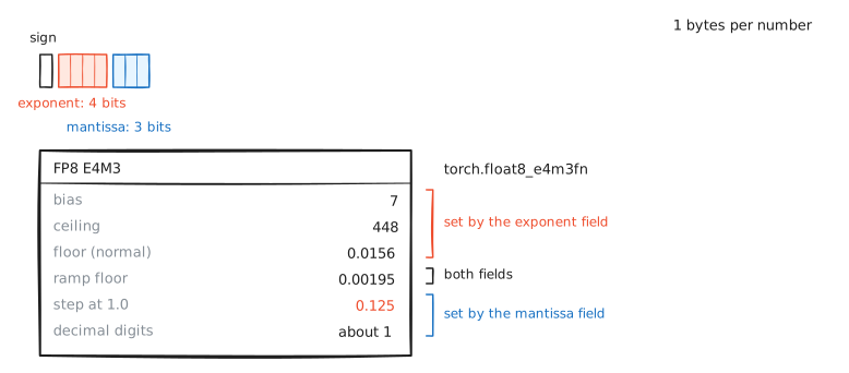
E4M3 you have known since the map section: its 15 intervals are this page's teaching map, and its 256 patterns are decoded in proof. The card records its one non-IEEE choice: no infinity. Those patterns were used for one more doubling of range, overflow stops at 448, and a single pattern means NaN.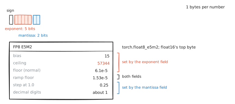
E5M2 is float16 with the bottom byte cut, and that is a bit-level fact, provable the same way bfloat16 was: all 256 E5M2 patterns cast to float16 as the same 8 bits with 8 zeros appended (proof checks every one).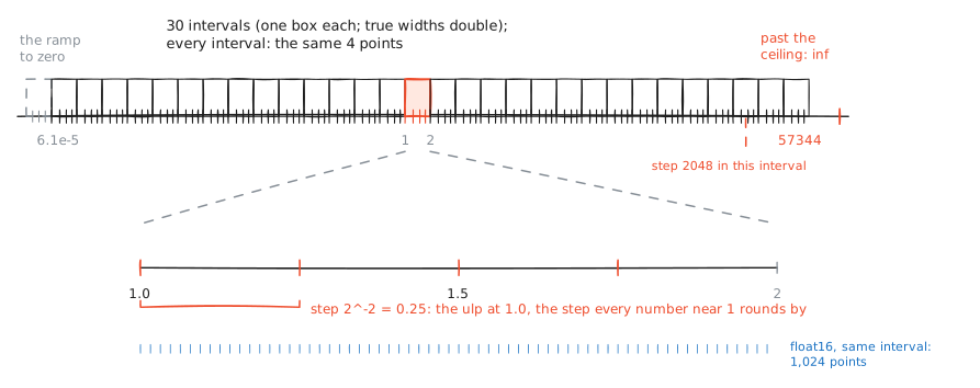
p20_e5m2_top_byte.py the proof, ready to read or run
download and run it# fp8 e5m2 is float16's top byte, at the bit level. the same fact
# as bfloat16 being float32's top half, one floor down: e5m2 keeps
# float16's 5 exponent bits and the top 2 of its 10 mantissa bits.
# cast any of the 256 e5m2 bit patterns to float16 and the result
# is the same 8 bits with 8 zeros appended.
import torch
pats = torch.arange(256, dtype=torch.uint8)
as_e5m2 = pats.view(torch.float8_e5m2)
up_bits = as_e5m2.half().view(torch.int16) & 0xFFFF
want = pats.to(torch.int16) << 8
nan_mask = torch.isnan(as_e5m2)
ok = (up_bits == want) | nan_mask
print(f"up-cast bit check: {ok.sum().item()} / 256 patterns match "
f"(pattern << 8)")
print(f" {nan_mask.sum().item()} NaN patterns, all up-cast to "
f"float16 NaN: {torch.isnan(as_e5m2.half()[nan_mask]).all().item()}")
exact = (up_bits == want).sum().item()
print(f" bit-exact including NaN payloads: {exact} / 256")
# the picture, on one number
v = torch.tensor(1.7014, dtype=torch.float16)
b8 = v.to(torch.float8_e5m2).view(torch.uint8).item()
u16 = v.view(torch.int16).item() & 0xFFFF
print(f"\n1.7014 in float16 bits: {u16:016b}")
print(f"1.7014 in E5M2 bits : {b8:08b} (the top byte, rounded)")
print(f"E5M2 value stored : "
f"{v.to(torch.float8_e5m2).float().item():.4f}")
# the run prints:
#
# up-cast bit check: 256 / 256 patterns match (pattern << 8)
# 6 NaN patterns, all up-cast to float16 NaN: True
# bit-exact including NaN payloads: 254 / 256
#
# 1.7014 in float16 bits: 0011111011001110
# 1.7014 in E5M2 bits : 00111111 (the top byte, rounded)
# E5M2 value stored : 1.7500
#
# all 256 patterns check out; the 2 that are not bit-exact are nan
# patterns whose payload bits torch is free to place differently,
# and both still arrive as float16 nans. the down-cast of 1.7014
# keeps the top byte and rounds by the dropped 8 bits, landing on
# 1.75: the same truncation bfloat16 performs on float32.
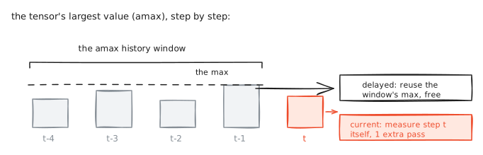
NVIDIA, Arm and Intel proposed the pair for deep learning in 2022 [6], and hardware arrived with the Hopper chips. In use, E4M3 carries the forward pass. E5M2 carries the gradients, whose thin far tails need reach more than digits. And one more piece rides along: every FP8 tensor gets one float32 scale of its own. The scale is picked from the tensor's recent largest value, so that the tensor's histogram slides into the band. This is exactly the loss-scaling move, now made automatic and applied per tensor. Recipes differ only in when they measure that largest value: from recent history (delayed scaling) or on the spot (current scaling):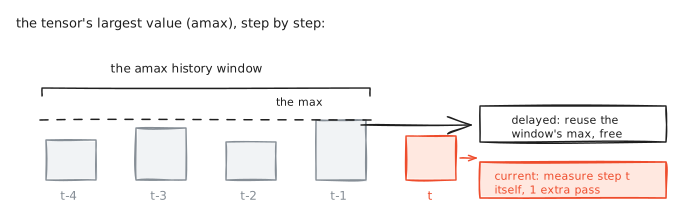
And not everything is quantized. (To quantize a tensor: move its numbers onto a narrower format's points.) Attention's and the MLP's big matmuls run in FP8. Softmax, the normalizations, the first embedding and the final projection stay wide [11].
Wired into a transformer through NVIDIA's Transformer Engine, the published result is training 30 to 40 percent faster at matching loss curves [6]. DeepSeek-V3 pushed the same idea one step finer: it trained a 671-billion-parameter model with FP8 matmuls by giving a scale to every 128-element tile instead of every tensor [7]. Hold that thought; it is halfway to the next section. And one honest caution before the next halving. E4M3 carries about 1.2 decimal digits. E5M2 carries about 0.9. At 8 bits, no single stored number is trustworthy. Only averages over many are.
The outlier problem
Before the next halving, meet the format waiting at the bottom, because its 2 numbers explain everything that follows. 4 bits: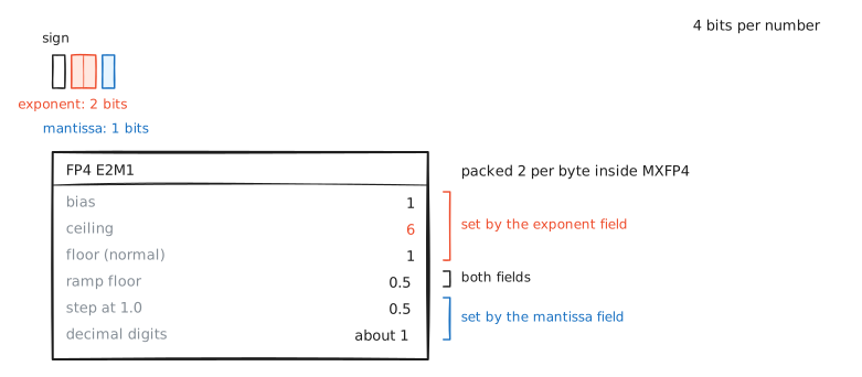
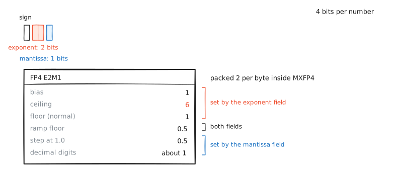
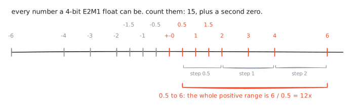
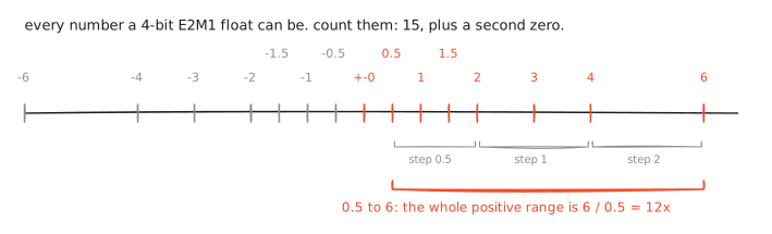
16 patterns. 15 values (0 appears twice, once with each sign). No inf, no NaN. And one number to hold on to: the whole positive range is 6 / 0.5 = 12x, about 3.6 doublings. The 2023 OCP standard defined E2M1 as the 4-bit element of the block family these sections are building [9], and the newest NVIDIA chips run it at twice the FP8 rate [24]. But alone it is unusable. Even the per-tensor scale that carried FP8 cannot save it, because per-tensor scaling has one enemy. Transformer activations grow a few channels whose values run hundreds of times larger than the rest, systematically, past about 6 billion parameters [8]. One scale must now serve the spike and the bell at once: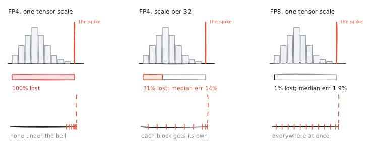
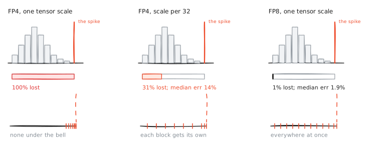
Read the measured numbers. FP8 with a single scale loses 1% of the ordinary values next to a 500x outlier, because a float grid keeps its relative error at any scale until values fall below its smallest positive number, and FP8's smallest is 229,376x under its largest (448 / 0.00195, from the map section). FP4's smallest is only 12x under its largest (6 / 0.5, computed above). One spike takes the whole 12x, and 100% of the ordinary values quantize to zero (proof). At 4 bits, blocks are not an improvement; nothing works without them.
p10_fp4_outlier.py the proof, ready to read or run
download and run it# why blocks had to be invented.
#
# a float grid keeps its relative precision at any scale, so fp8
# with one per-tensor scale survives an outlier surprisingly well.
# fp4 does not: its largest positive value is 6 and its smallest is
# 0.5, only 12x apart, so one spike pushes every ordinary value
# below the smallest and the tensor quantizes to zeros. a scale per
# 32 elements rescues it.
import torch
E2M1 = torch.tensor([0.0, 0.5, 1.0, 1.5, 2.0, 3.0, 4.0, 6.0])
def round_e2m1(v):
# nearest e2m1 magnitude, sign restored after
idx = (v.abs().unsqueeze(-1) - E2M1).abs().argmin(-1)
return E2M1[idx] * v.sign()
def quant(x, block):
# one absmax scale per block, elements rounded onto e2m1
q = torch.empty_like(x)
for i in range(0, len(x), block):
b = x[i:i+block]
s = b.abs().max() / 6.0
s = s if s > 0 else torch.tensor(1.0)
q[i:i+block] = round_e2m1(b / s) * s
return q
torch.manual_seed(0)
x = torch.randn(128) * 0.1 # ordinary values near 0.1
x[40] = 50.0 # one spike, 500x the rest
mask = torch.ones(128, dtype=torch.bool); mask[40] = False
for name, block in (("per-tensor", 128), ("per-block-32", 32)):
q = quant(x, block)
zeros = (q[mask] == 0).float().mean()
rel = ((q - x)[mask].abs() / x[mask].abs()).median()
print(f"{name:14s} ordinary values quantized to zero: {zeros:.0%} "
f"median rel err of the rest: {rel:.1%}")
q = quant(x, 128)
print(f"the outlier itself survives either way: {q[40]:.1f}")
print()
print("the same tensor in FP8 E4M3, one per-tensor scale, for honesty:")
s = x.abs().max() / 448.0
q8 = (x / s).to(torch.float8_e4m3fn).float() * s
print(f"per-tensor FP8 zeros: {(q8[mask]==0).float().mean():.0%} "
f"median rel err: {((q8-x)[mask].abs()/x[mask].abs()).median():.1%}")
print("a float grid holds its relative error at any scale, until its")
print("smallest positive value; FP4's smallest (0.5) is only 12x below")
print("its largest (6), and that is the whole reason microscaling exists.")
# the run prints (seeded):
#
# per-tensor ordinary values quantized to zero: 100% median rel err of the rest: 100.0%
# per-block-32 ordinary values quantized to zero: 31% median rel err of the rest: 14.2%
# the outlier itself survives either way: 50.0
#
# the same tensor in FP8 E4M3, one per-tensor scale, for honesty:
# per-tensor FP8 zeros: 1% median rel err: 1.9%
#
# with one scale for the whole tensor, fp4 keeps the spike and
# turns 100% of the other 127 values into zeros. cutting the scale's
# reach to 32 elements confines the damage to the spike's own block,
# and fp8 with its 448/0.002 span barely notices the spike at all.
Microscaling
So the scale moved into the data type. The Open Compute Project's MX formats, standardized in 2023 by AMD, Arm, Intel, Meta, Microsoft, NVIDIA and Qualcomm [9], cut every tensor into blocks of 32 and give each block one 8-bit scale: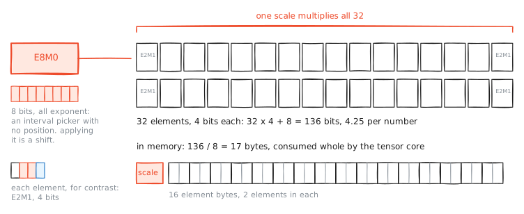
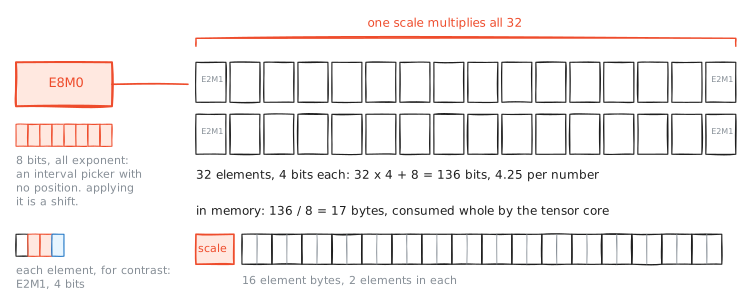
Every idea on this page meets here, so take it slowly. The scale byte is an E8M0: a float with no mantissa at all. It is the interval-picker from the floating-dot figure with the position deleted, so applying it is just exponent addition, nearly free in silicon. The block of 32 is the histogram idea cut fine: an outlier can now only hurt its own 31 neighbors. The price is small. 32 x 4 + 8 = 136 bits for 32 numbers, 4.25 bits each; 136 / 128 = 1.06, so 6% over raw 4-bit storage. Even the block size is a measured compromise: smaller blocks fit better but spend more bits on scales, and our own sweep across sizes 8, 16, 32, 64 and 128 shows both effects moving (proof). The same block layout carries 8-, 6- and 4-bit elements, named MXFP8, MXFP6, MXFP4.
What the tensor core does with 2 of these blocks is 1 more drawing: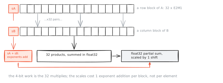
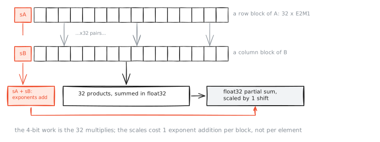
The block layout also changed who does what inside FP8. With a scale for every 32 values, one block rarely spans more than E4M3's 18 doublings. So E4M3, which has 8 points per doubling where E5M2 has 4, measured better for the gradients too. The largest published MXFP8 pretraining run, 8 billion parameters on 15 trillion tokens, quantizes every tensor as E4M3 [11].
The 6-bit elements deserve their own cards, because they are the family's open seats: E2M3 keeps digits, E3M2 keeps reach, one more run of the fork.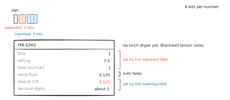
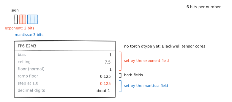
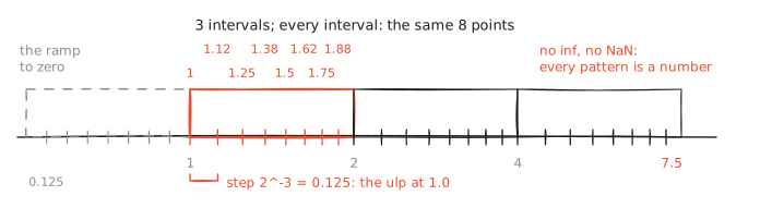
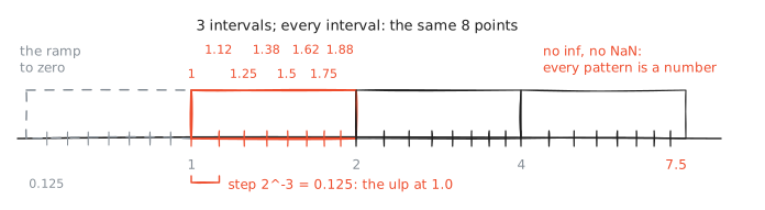
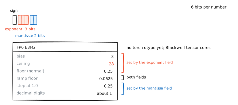
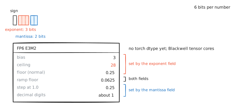
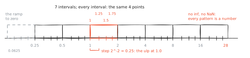
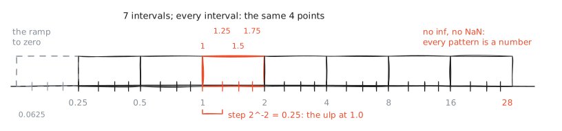
Their maps are small enough to draw complete: 3 intervals of 8 points, 7 intervals of 4. Blackwell-class chips execute them at full speed as MXFP6 [9][24]; almost no published recipe uses them yet. A format survives by having a job nobody else does. FP8 is safer, FP4 is faster on paper, and FP6 is still looking for its job.
NVIDIA's NVFP4 variant tightens it further: 16-element blocks, a fractional E4M3 scale instead of a power-of-two one, plus one float32 scale per tensor, buying a finer fit for a quarter bit more [10]. The bytes carry the quarter bit, and the deeper difference sits in the scale byte itself: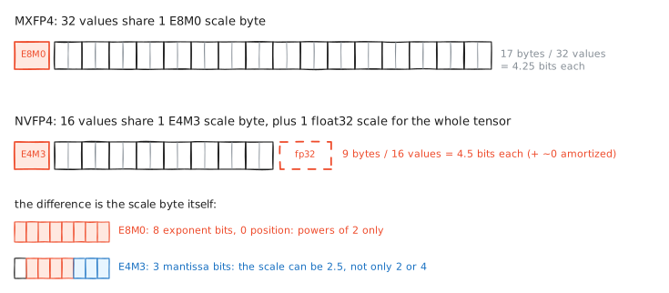
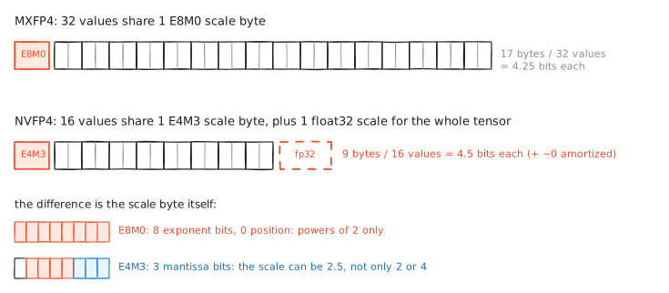
Here is one NVFP4 block quantized by hand, every scale shown: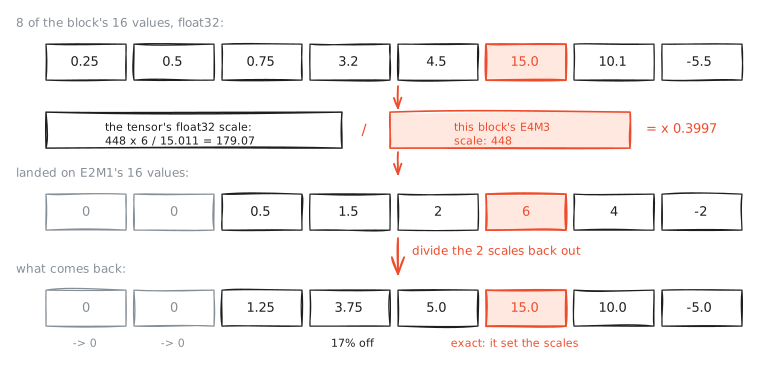
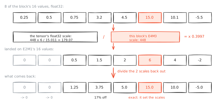
The largest of the 16 values, 15.011, sets the scales and comes back exactly; 0.25 and 0.5 fall below half of the smallest step at that scale and come back as 0; 3.2002 comes back as 3.7528, about 17% off (proof runs every number). A single 4-bit value is coarse. The bet of 4-bit arithmetic is that billions of such errors, kept unbiased, cancel on average.
p19_nvfp4_worked.py the proof, ready to read or run
download and run it# one nvfp4 block, quantized by hand, every scale shown.
#
# re-derives the worked 1 x 16 example from nvidia's recipe (as
# walked through by radical numerics): a global float32 scale
# brings the tensor's largest value into range, each 16-value block
# gets an fp8 e4m3 scale, and the elements land on the 16 values
# of e2m1.
import torch
E2M1_MAX = 6.0
E4M3_MAX = 448.0
BLOCK = 16
E2M1_GRID = torch.tensor([0.0, 0.5, 1.0, 1.5, 2.0, 3.0, 4.0, 6.0])
def rne_e2m1(x):
# nearest e2m1 value, both signs in one grid
grid = torch.cat([E2M1_GRID, -E2M1_GRID.flip(0)])
d = (x.unsqueeze(-1) - grid).abs()
return grid[d.argmin(dim=-1)]
x = torch.tensor([0.0, 0.25, 0.5, 0.75356, 1.251245, 3.2002,
4.5032, 15.011, 0.012, -0.312, -5.50055, 10.06,
-1.2526, 3.025, 2.5114, 7.0162])
# level 1: one float32 scale for the whole tensor
global_amax = x.abs().max()
s_enc = (E4M3_MAX * E2M1_MAX) / global_amax
s_dec = 1.0 / s_enc
# level 2: one e4m3 scale for each block of 16
block_amax = x.abs().max() # one block here, so same amax
dec_scale = (block_amax / E2M1_MAX) * s_enc
dec_scale_e4m3 = dec_scale.to(torch.float8_e4m3fn)
enc_scale = 1.0 / (dec_scale_e4m3.float() * s_dec)
print(f"level 1, the tensor's float32 scale: 448 x 6 / "
f"{global_amax:.4f} = {s_enc:.2f}")
print(f"level 2, this block's E4M3 scale: "
f"{dec_scale_e4m3.float():g}")
print(f"together: {s_enc:.2f} / {dec_scale_e4m3.float():g} = "
f"{enc_scale:.4f}, the factor every value is multiplied by")
# quantize: scale, clamp to e2m1's range, round onto its 16 values
scaled = (x * enc_scale).clamp(-E2M1_MAX, E2M1_MAX)
q = rne_e2m1(scaled)
# dequantize: multiply back by both scales
dq = q * dec_scale_e4m3.float() * s_dec
print(f"global amax {global_amax:.4f} block encode scale "
f"{enc_scale:.4f}\n")
print(f"{'input':>9s} {'scaled':>8s} {'E2M1':>6s} {'back':>9s}")
for a, b, c, d in zip(x, scaled, q, dq):
print(f"{a:>9.4f} {b:>8.4f} {c:>6.1f} {d:>9.4f}")
print("\nread the two ends: 15.011 comes back as 15.011 exactly")
print("(it set the scales), 0.25 and 0.5 come back as 0 (they")
print("fell below half of E2M1's smallest step at this scale),")
print("3.2002 comes back as 3.7528: about 17% off. one 4-bit")
print("number is coarse; the training recipe works because these")
print("errors average out over billions of them.")
# the run prints:
#
# level 1, the tensor's float32 scale: 448 x 6 / 15.0110 = 179.07
# level 2, this block's E4M3 scale: 448
# together: 179.07 / 448 = 0.3997, the factor every value is multiplied by
# global amax 15.0110 block encode scale 0.3997
#
# input scaled E2M1 back
# 0.0000 0.0000 0.0 0.0000
# 0.2500 0.0999 0.0 0.0000
# 0.5000 0.1999 0.0 0.0000
# 0.7536 0.3012 0.5 1.2509
# 1.2512 0.5001 0.5 1.2509
# 3.2002 1.2791 1.5 3.7527
# 4.5032 1.8000 2.0 5.0037
# 15.0110 6.0000 6.0 15.0110
# 0.0120 0.0048 0.0 0.0000
# -0.3120 -0.1247 0.0 0.0000
# -5.5005 -2.1986 -2.0 -5.0037
# 10.0600 4.0211 4.0 10.0073
# -1.2526 -0.5007 -0.5 -1.2509
# 3.0250 1.2091 1.0 2.5018
# 2.5114 1.0038 1.0 2.5018
# 7.0162 2.8044 3.0 7.5055
#
# the 2 scale levels multiply into one factor, 0.3997, and the
# largest value maps to exactly 6.0, the top of e2m1's range, and
# comes back without loss. everything else lands on the nearest of
# 16 coarse values, and 0.25 and 0.5 fall through to zero.
One subtlety earned a hardware rule. The E8M0 scale can only be a power of 2, so a block whose largest value is 5.9 must round its scale one way or the other, and the 2 ways are not close: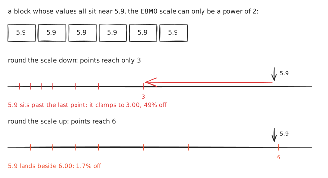
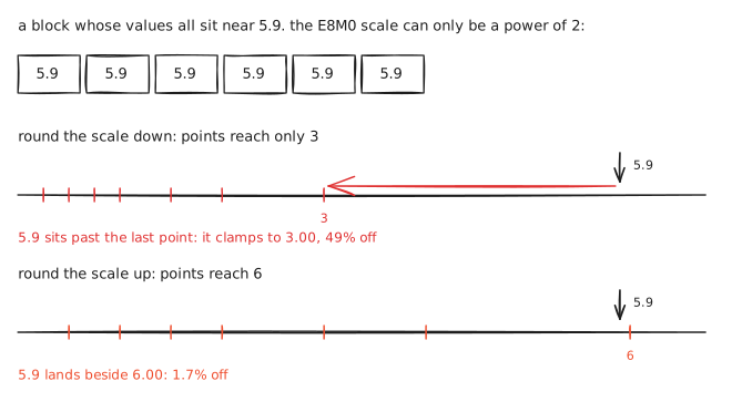
NVIDIA measured the difference as the gap between divergence and parity at trillion-token scale [11]; proof shows the mechanism in 2 lines.
The whole scaling story now fits on one ladder, and every recipe of the last 5 sections is 1 rung of it: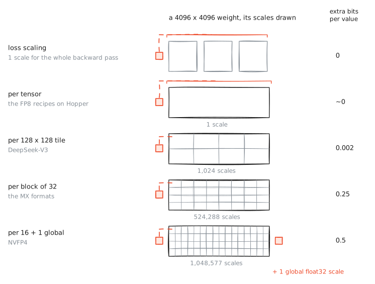
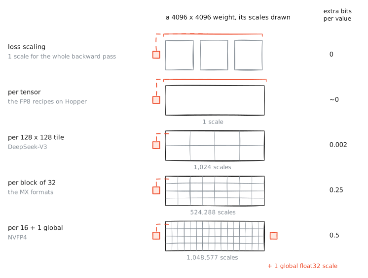
Training at 4 bits
The destination format, E2M1, was drawn whole 2 sections back: 15 values, 12x wide. Training inside those 16 patterns needs 3 rescues beyond blocks, and each is an idea from earlier on this page pushed one step:
The first is stochastic rounding, the lost-update repair now doing the main work. At 4 bits nearly every update is below half the local step, so deterministic rounding freezes everything; rounding up with probability proportional to progress is unbiased in expectation. Our proof runs 10,000 micro-updates: nearest rounds to a frozen 1.0, stochastic reaches a mean of 3.0113 against a true 3.0, noisy per run and honest on average (proof).
p12_sr_drift.py the proof, ready to read or run
download and run it# round-to-nearest is biased when every step is smaller than half
# the local spacing; stochastic rounding is unbiased in expectation.
# the same fact that froze the bf16 weight in the lost-update
# proof, isolated and repeated 50 times.
import torch
N, u, TRIALS = 10000, 2e-4, 50 # each step is about 1/39 of bf16's step at 1.0
def sr_walk(seed):
# add u N times, rounding to a bf16 neighbor with probability
# proportional to how far the true value sits between them
g = torch.Generator().manual_seed(seed)
val = 1.0
for _ in range(N):
x = val + u
lo = torch.tensor(x, dtype=torch.bfloat16)
lo_f = lo.float().item()
hi_f = torch.nextafter(lo, torch.tensor(float("inf"), dtype=torch.bfloat16)).float().item()
if lo_f > x: # x landed below its rounded value
hi_f, lo_f = lo_f, torch.nextafter(lo, torch.tensor(float("-inf"), dtype=torch.bfloat16)).float().item()
p = 0.0 if hi_f == lo_f else (x - lo_f) / (hi_f - lo_f)
val = hi_f if torch.rand((), generator=g).item() < p else lo_f
return val
# the deterministic walk: round-to-nearest rounds every step away
rne = torch.tensor(1.0, dtype=torch.bfloat16)
for _ in range(N):
rne = rne + torch.tensor(u, dtype=torch.bfloat16)
finals = torch.tensor([sr_walk(s) for s in range(TRIALS)])
true = 1.0 + N * u
print(f"true value : {true:.4f}")
print(f"round-to-nearest, {N} steps : {rne.item():.4f} (frozen)")
print(f"stochastic rounding, {TRIALS} runs : "
f"mean {finals.mean().item():.4f}, spread +-{finals.std().item():.4f}")
print("unbiased in expectation, noisy per run: that is the trade.")
# the run prints (seeded):
#
# true value : 3.0000
# round-to-nearest, 10000 steps : 1.0000 (frozen)
# stochastic rounding, 50 runs : mean 3.0113, spread +-0.1384
#
# 10000 additions that should carry 1.0 up to 3.0. round-to-nearest
# refuses every one of them and ends where it started. stochastic
# rounding takes an occasional full step up, in just the right
# proportion: across 50 runs the mean lands on 3.01, each single
# run wandering by about 0.14 around it.
The second is the random Hadamard transform: rotate the tensor by an orthogonal matrix before quantizing and undo it after, which changes no matmul (the rotation cancels) but spreads an outlier's energy across every coordinate: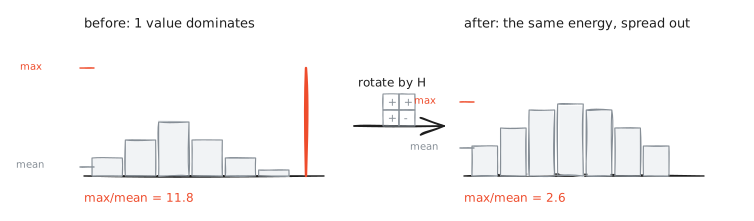
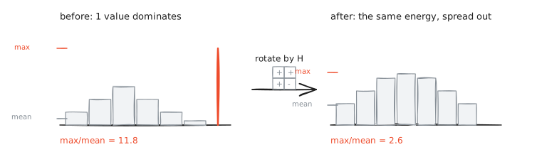
Our 64-value proof takes the max-to-mean ratio from 11.8 to 2.6 (proof). The third is selective precision: the first and last layers, where quantization error is measured to hurt most, stay in higher precision. With all three plus NVFP4, a 12-billion-parameter model has been pretrained on 10 trillion tokens at nearly the same loss as its FP8 twin [10]; MXFP4 needs more tokens for the same loss [12]. Where each rescue is applied is itself measured engineering [10][24]. Stochastic rounding runs only on the gradients; on the forward pass it would add noise for nothing, so weights and activations round to nearest. The Hadamard rotation runs only on the inputs of the weight-gradient matmul. And weights are scaled in 16 x 16 squares rather than 1 x 16 rows, for a reason worth drawing: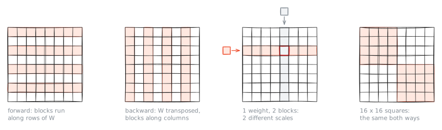
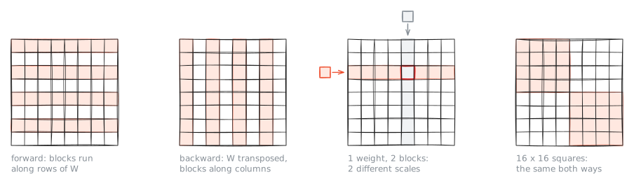
A row-scaled weight matrix and its column-scaled transpose are 2 different quantized matrices, and the forward and backward passes must see the same weights. The last roughly 15% of layers stay in higher precision, and if a gap to the wide baseline remains at the end, switching the forward pass to higher precision for the final phase of training closes most of it [10][24]. 4-bit training is real and it is young; treat recipes as versioned, not settled.
p13_hadamard.py the proof, ready to read or run
download and run it# an orthogonal rotation spreads one outlier's energy across every
# coordinate, without changing the vector's length or the matmul it
# feeds (H is orthogonal, so H @ H.T is the identity and it can be
# undone on the other side). the max shrinks; the format's points
# get used again.
import torch
def hadamard(n):
# the classic doubling construction: H_2n = [[H, H], [H, -H]],
# scaled by 1/sqrt(2) each doubling to stay orthonormal
H = torch.tensor([[1.0]])
while H.shape[0] < n:
H = torch.cat([torch.cat([H, H], 1), torch.cat([H, -H], 1)], 0) / (2 ** 0.5)
return H
torch.manual_seed(3)
n = 64
x = torch.randn(n) * 0.5
x[7], x[23], x[51] = 8.0, -7.0, 6.0 # 3 planted outliers
H = hadamard(n)
y = x @ H
print(f"norm preserved: {torch.allclose(x.norm(), y.norm())}")
for name, v in (("before", x), ("after H", y)):
print(f"{name:8s} max {v.abs().max():.3f} mean {v.abs().mean():.3f} "
f"max/mean {(v.abs().max()/v.abs().mean()).item():.2f}")
# the run prints (seeded):
#
# norm preserved: True
# before max 8.000 mean 0.678 max/mean 11.80
# after H max 3.438 mean 1.336 max/mean 2.57
#
# the length of the vector did not move, but the spike shrank from
# 8.0 to 3.4 and the max-to-mean ratio fell from 11.8 to 2.6. a
# per-block scale is now set by ordinary values instead of by the
# spike alone; that is the move inside quip#, quarot, and
# spinquant.
The other grids
Inference relaxed one constraint: if only the weights are quantized and arithmetic runs wider, the 16 points need not be a float at all. 3 designs compete on the same bell-shaped distribution of trained weights: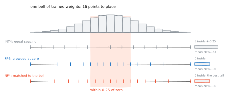
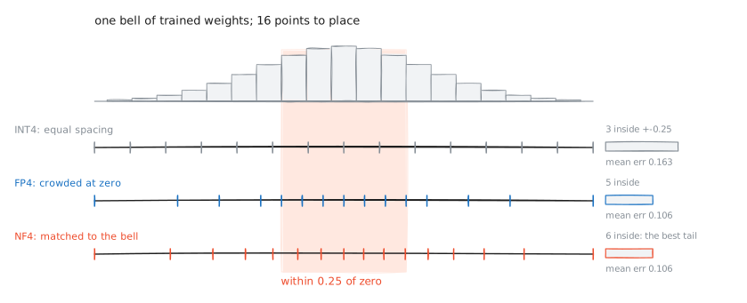
INT4 spaces its points equally, so it wastes points where weights are rare. FP4 doubles its steps and crowds zero. NF4, from the QLoRA work, places its 16 values at the quantiles of a gaussian, which is approximately what trained weights are, and it wins the tail (proof, [13]). Around these grids grew the post-training toolkit, one idea per tool. GPTQ rounds each weight so as to compensate the error left by the weights before it [14]. AWQ rescales channels so the few weights that matter most land on finer points [15]. And the same how-many-bits question now runs through the KV cache, and even the optimizer states: an 8-bit Adam keeps its moments in blocks with per-block scales [16], the MX idea arriving from the other direction.
p14_grids.py the proof, ready to read or run
download and run it# 3 ways to spend 16 points.
#
# int4's uniform grid, fp4 e2m1's doubling grid, and nf4's quantile
# grid (the 16 values from the qlora paper), each quantizing the
# same 100,000 gaussian weights with one absmax scale.
import torch
torch.manual_seed(0)
w = torch.randn(100_000)
INT4 = torch.linspace(-7, 7, 15) / 7.0 # uniform, symmetric
E2M1 = torch.tensor([0.0, 0.5, 1.0, 1.5, 2.0, 3.0, 4.0, 6.0]) / 6.0
E2M1 = torch.cat([-E2M1.flip(0), E2M1]).unique() # both signs, one zero
NF4 = torch.tensor([-1.0, -0.6961928009986877, -0.5250730514526367,
-0.39491748809814453, -0.28444138169288635, -0.18477343022823334,
-0.09105003625154495, 0.0, 0.07958029955625534, 0.16093020141124725,
0.24611230194568634, 0.33791524171829224, 0.44070982933044434,
0.5626170039176941, 0.7229568362236023, 1.0]) # dettmers et al. 2023
s = w.abs().max()
for name, grid in (("INT4 uniform", INT4), ("FP4 E2M1", E2M1),
("NF4 quantile", NF4)):
q = grid[( (w / s).unsqueeze(-1) - grid ).abs().argmin(-1)] * s
err = (q - w).abs()
print(f"{name:14s} mean abs err {err.mean():.4f} "
f"p99 {err.quantile(0.99):.4f}")
print("\nmost gaussian weights sit near zero; NF4 spends its 16 points there.")
# the run prints (seeded):
#
# INT4 uniform mean abs err 0.1626 p99 0.3226
# FP4 E2M1 mean abs err 0.1064 p99 0.3495
# NF4 quantile mean abs err 0.1060 p99 0.2514
#
# the uniform grid wastes points out in the tails where almost no
# weight lives. e2m1's doubling steps crowd points near zero and
# cut the mean error by a third, at the cost of a worse 99th
# percentile. nf4, built from the gaussian's own quantiles, matches
# e2m1 on the mean and beats everything on the tail.
The whole family on one sheet
Every format on this page has now been met. Gather them: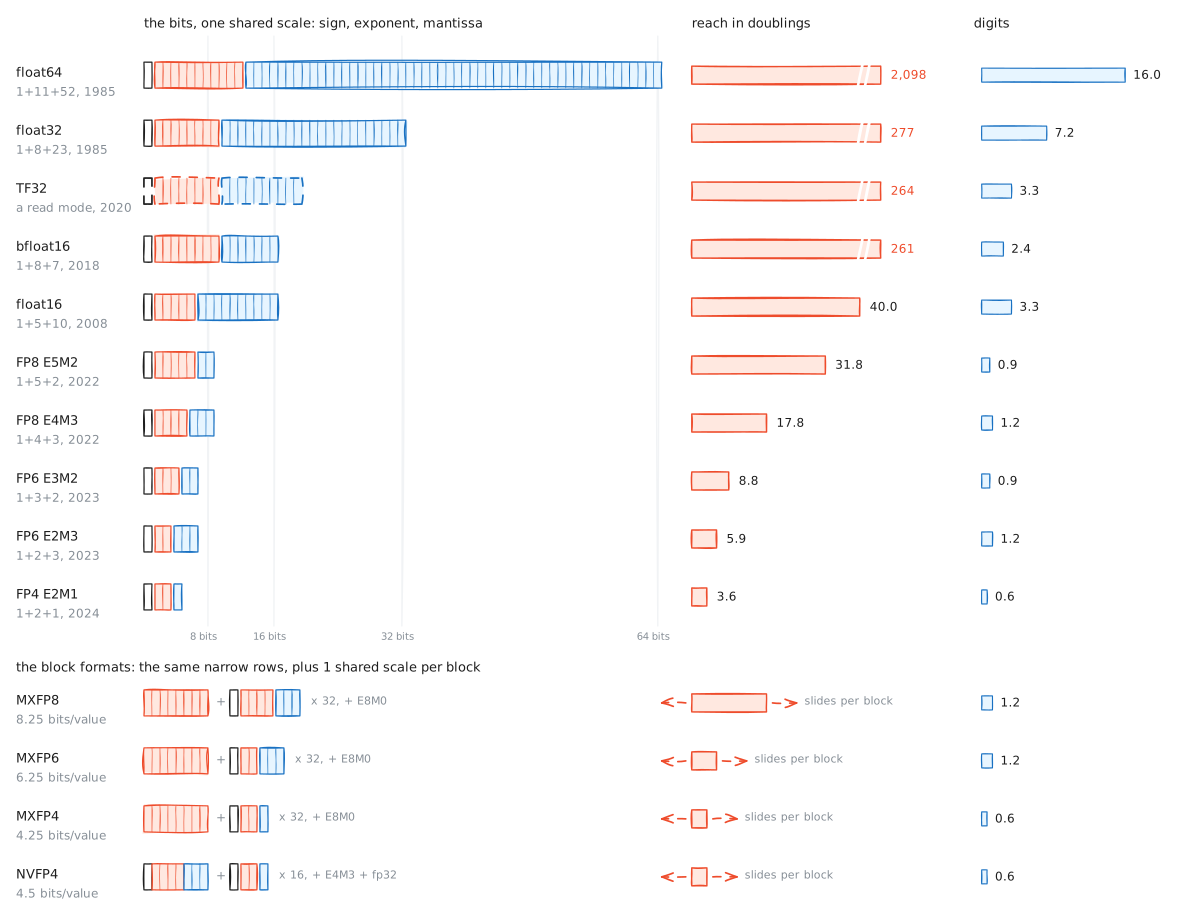
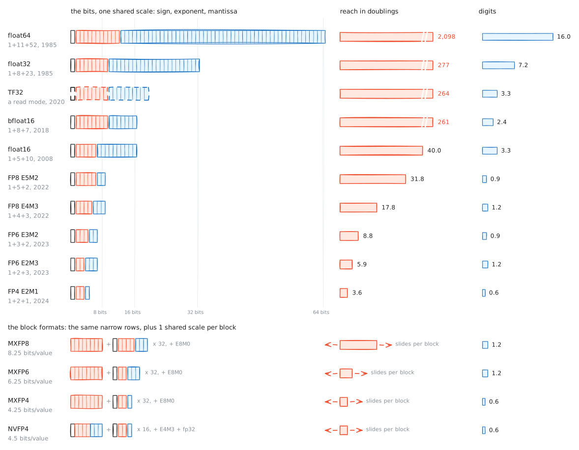
p18_family_sheet.py the proof, ready to read or run
download and run it# the whole-family sheet, derived from each format's bit counts and
# checked against torch wherever torch has the type.
#
# for every format: ceiling, smallest positive value, the number of
# doublings between them (log2 of their ratio), step at 1.0, and
# decimal digits. kind says how the top exponent patterns are used:
#
# ieee top exponent pattern reserved for inf and nan
# fn no inf; only the top mantissa pattern of the top exponent
# is nan (fp8 e4m3)
# all no inf and no nan; every pattern is a number (fp4 e2m1,
# both fp6 shapes)
import math
import torch
def family(E, M, bias, kind):
if kind == "ieee":
emax = 2 ** E - 2 - bias # top pattern lost to inf/nan
ceiling = (2 - 2.0 ** -M) * 2.0 ** emax
elif kind == "fn":
emax = 2 ** E - 1 - bias # top pattern kept, minus its nan
ceiling = (2 - 2.0 ** (1 - M)) * 2.0 ** emax
else: # all
emax = 2 ** E - 1 - bias # every pattern is a number
ceiling = (2 - 2.0 ** -M) * 2.0 ** emax
smallest = 2.0 ** (1 - bias - M) # smallest subnormal
return {
"ceiling": ceiling,
"smallest": smallest,
"doublings": math.log2(ceiling) - math.log2(smallest),
"step1": 2.0 ** -M,
"digits": (M + 1) * math.log10(2),
}
ROWS = [
("float64", 11, 52, 1023, "ieee", torch.float64),
("float32", 8, 23, 127, "ieee", torch.float32),
("TF32", 8, 10, 127, "ieee", None),
("bfloat16", 8, 7, 127, "ieee", torch.bfloat16),
("float16", 5, 10, 15, "ieee", torch.float16),
("FP8 E5M2", 5, 2, 15, "ieee", torch.float8_e5m2),
("FP8 E4M3", 4, 3, 7, "fn", torch.float8_e4m3fn),
("FP6 E3M2", 3, 2, 3, "all", None),
("FP6 E2M3", 2, 3, 1, "all", None),
("FP4 E2M1", 2, 1, 1, "all", None),
]
print(f"{'format':10s} {'ceiling':>10s} {'smallest':>10s} "
f"{'doublings':>9s} {'step at 1':>10s} {'digits':>6s}")
for name, E, M, bias, kind, dt in ROWS:
f = family(E, M, bias, kind)
print(f"{name:10s} {f['ceiling']:>10.4g} {f['smallest']:>10.3g} "
f"{f['doublings']:>9.1f} {f['step1']:>10.4g} "
f"{f['digits']:>6.1f}")
if dt is not None:
fi = torch.finfo(dt)
assert f["ceiling"] == fi.max, (name, f["ceiling"], fi.max)
assert f["step1"] == fi.eps, (name, f["step1"], fi.eps)
print("\ntorch.finfo agrees on ceiling and step for every format "
"torch carries\n(float64/32/16, bfloat16, both FP8 types).")
print("FP6 sheets from the same formulas; Blackwell tensor cores "
"run them,\ntorch has no storage type for them yet.")
# the run prints (torch 2.11.0):
#
# format ceiling smallest doublings step at 1 digits
# float64 1.798e+308 4.94e-324 2098.0 2.22e-16 16.0
# float32 3.403e+38 1.4e-45 277.0 1.192e-07 7.2
# TF32 3.401e+38 1.15e-41 264.0 0.0009766 3.3
# bfloat16 3.39e+38 9.18e-41 261.0 0.007812 2.4
# float16 6.55e+04 5.96e-08 40.0 0.0009766 3.3
# FP8 E5M2 5.734e+04 1.53e-05 31.8 0.25 0.9
# FP8 E4M3 448 0.00195 17.8 0.125 1.2
# FP6 E3M2 28 0.0625 8.8 0.25 0.9
# FP6 E2M3 7.5 0.125 5.9 0.125 1.2
# FP4 E2M1 6 0.5 3.6 0.5 0.6
#
# one function, 10 formats. read the doublings column top to
# bottom: 2098, 277, 264, 261, 40, 31.8, 17.8, 8.8, 5.9, 3.6.
# that shrinking number is the entire story of the article, in a
# single column.
Read the sheet by columns. The bit bars share one scale: you can see float64 dwarf everything and the narrow rows shrink to almost nothing. The reach bars collapse from float64's 2,098 doublings to E2M1's 3.6; every format from float16 down fits its whole reach on the drawing. The digits column falls from 16 to 0.6. The block rows at the bottom are the repair: the same narrow elements, plus a shared scale whose dashed arrows say what it does, sliding each block's small reach to wherever its values live. And the sheet is the page in one drawing: everything before the field guide taught you what the columns mean, and everything after it was the story of how the narrow rows are made usable.
Where the bytes live
All of it, on one shelf: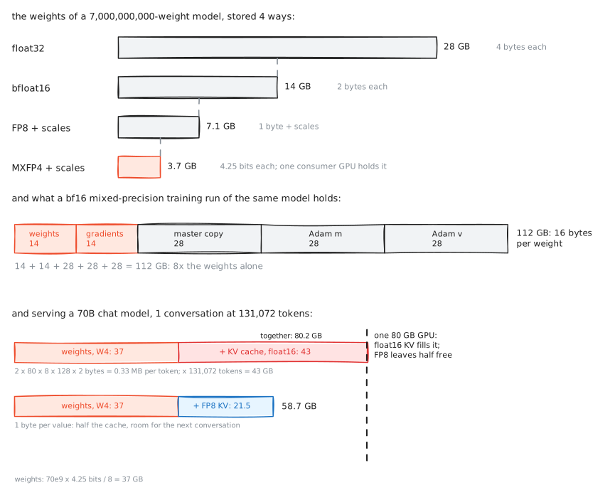
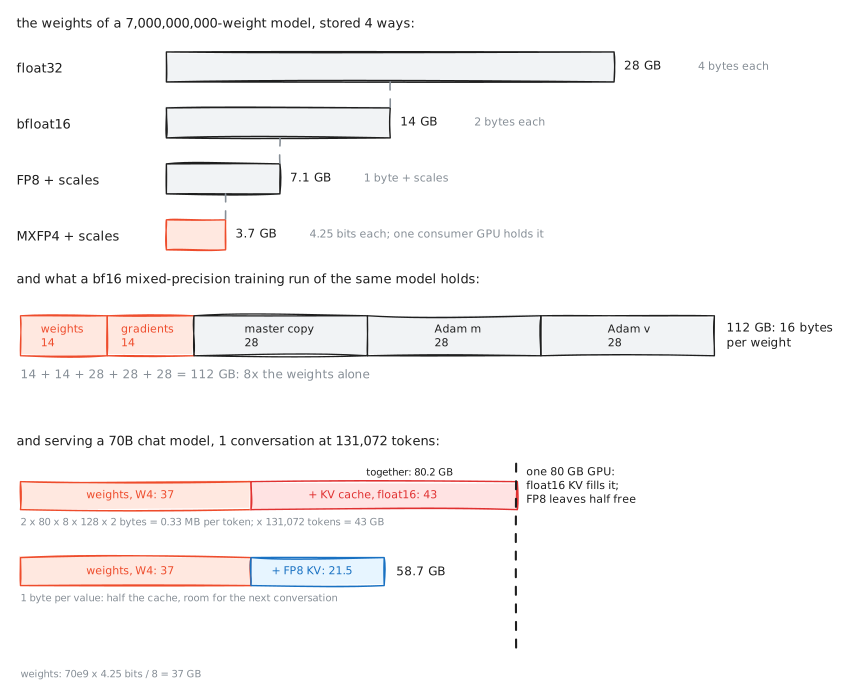
These panels are the honest reason this whole family of formats exists. A 7-billion-parameter model is 28 GB of float32 or 3.7 GB of MXFP4 with its scales; a training run holds 8x its bf16 weights; and in serving, the KV cache decides how many conversations one GPU carries. gpt-oss ships its 120-billion-parameter mixture-of-experts in MXFP4 so it fits a single 80 GB GPU [9].
Serving adds a loop of its own. A chat model generates 1 token at a time, and every token's step reads all the weights and the whole KV cache, the stored attention keys and values of every token so far; serving engines keep that cache in fixed-size pages so many conversations can grow side by side without fragmenting memory [29]. That loop, end to end: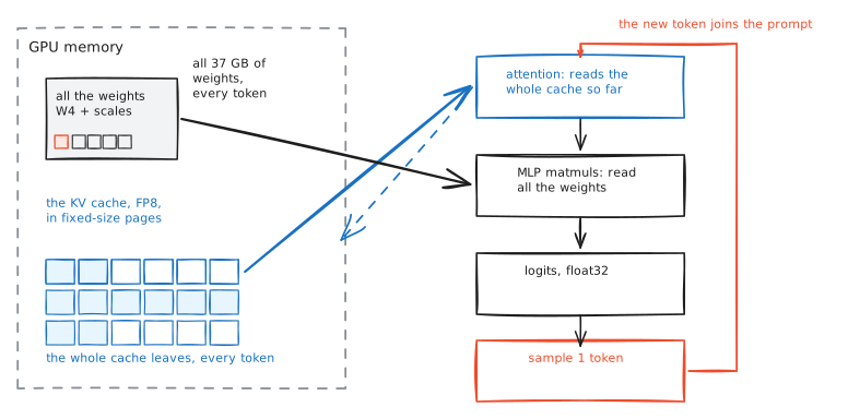
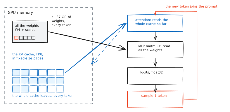
Hardware truth
Throughput follows the halvings only where the hardware speaks the format natively. On a GPU that must unpack a narrow format in software, the format saves memory but not time. That warning is measurable. One published comparison ran the same image-generation model on a GPU with no MXFP8 hardware. The MXFP8 file was smaller. Generation was slower than bfloat16: 112.8 seconds against 96.0, because every block had to be unpacked on the way in [25]. The same tests also ranked output quality: FP32 first, then FP16 and BF16 about equal, then MXFP8, then per-tensor-scaled FP8, then NVFP4, then plain FP8 last [25]. Size and quality move together, and a scale at any granularity beats no scale. Who speaks what natively today: NVIDIA's Blackwell chips run MXFP8/6/4 and NVFP4 in their tensor cores [24]; AMD's newest Instinct chips run the MX family [26]; Hopper GPUs and Trainium2 can store MX blocks but unpack them for the math [26]. The same facts, drawn so a spec sheet can be checked against them: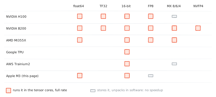
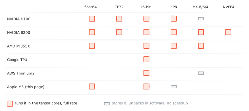
And what a native format buys, next to the measured price of one the hardware cannot speak: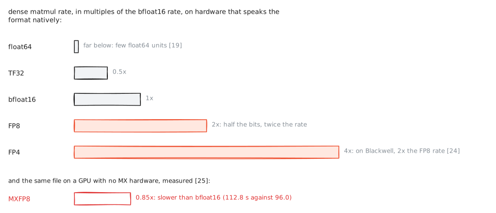
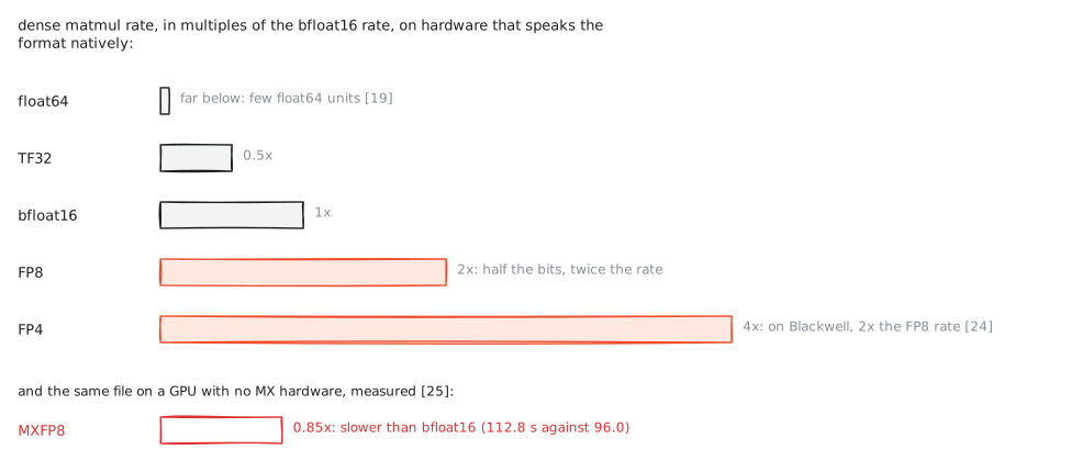
Read a spec sheet's format row before believing its speedup column.
The contract
Two runs of the same training script, same seeds, same data, on two different GPUs, will not match bit for bit. You now own every reason. Sums land in different orders on different core counts. Tensor cores round differently than the unfused loop. TF32 trims mantissas silently on one machine and not another. And there is a quieter actor: the compiler. IEEE 754 fixes each instruction's bits, but no language promises which instructions your line becomes. A compiler may legally fuse a * b + c into 1 fused multiply-add (1 rounding) or keep it as 2 instructions (2 roundings), and the choice can flip with an optimization flag or with something as small as inlining a function [27]; the rounding section's proof showed the 2 paths disagreeing. torch.compile is a compiler too: its fused kernels are allowed to round differently than eager mode [28]. And rounding in 2 hops is not rounding once: take an exact value to float64 first and then to float32, and you can land on a different number than going straight to float32, because the first rounding can create a tie the second one breaks the other way (proof builds one). This double rounding is why the old x87 unit, which computed in 80-bit registers and rounded again on every store to memory, made a program's bits depend on register allocation [4]. None of it is a bug; all of it is the map.
The same physics follows a model into serving. At temperature 0 an LLM should answer one prompt one way, and public endpoints do not: one measured run asked a model the same question 1,000 times and got 80 different answers [31]. The cause is not which GPU core finishes first; each kernel by itself returns the same bits every run. The cause is the batch. A server computes your request together with whoever else arrived, its kernels choose their splits, and so their addition order, by batch size, and a different order means different last bits. Other people's traffic changes your logits, and at some token the changed bits flip the chosen word. The repair is the one this page keeps teaching: pin the addition order. Kernels rewritten to reduce in one fixed pattern at every batch size made all 1,000 answers identical, at about a 2x cost in an unoptimized server [31].
p23_double_rounding.py the proof, ready to read or run
download and run it# rounding twice can differ from rounding once.
#
# take the exact value 1 + 2^-24 + 2^-60. rounded straight to
# float32 it goes up to 1 + 2^-23, because it sits just above the
# halfway point. rounded first to float64, the tiny 2^-60 tail is
# lost and the float64 result lands exactly on the halfway point;
# rounding that to float32 then goes down to 1.0 by ties-to-even.
# 2 legal paths, 2 different answers: double rounding, the failure
# mode of every system that computes wider first and stores
# narrower.
from fractions import Fraction as F
import numpy as np
exact = F(1) + F(1, 2 ** 24) + F(1, 2 ** 60)
# path 1: round once, straight to float32, decided with exact
# rational arithmetic so no float can cheat
lo, hi = F(1), F(1) + F(1, 2 ** 23) # the float32 neighbors
assert lo < exact < hi
once = np.float32(1.0) if (exact - lo) <= (hi - exact) else \
np.float32(1.0 + 2.0 ** -23)
# path 2: round to float64 first, then to float32
via64 = float(exact) # correctly rounded by python
twice = np.float32(via64)
print(f"exact value : 1 + 2^-24 + 2^-60")
print(f"rounded once to fp32 : {once!r}")
print(f"fp64 first : {via64!r}")
print(f"then to fp32 : {twice!r}")
assert once == np.float32(1.0 + 2.0 ** -23)
assert twice == np.float32(1.0)
print("\nthe 2 paths disagree. the old x87 unit computed in 80-bit")
print("registers and rounded again on every spill to memory, so a")
print("program's bits depended on register allocation; SSE and its")
print("one-width successors retired the problem, and this proof is")
print("why narrow-then-narrower casts still deserve suspicion.")
# the run prints:
#
# exact value : 1 + 2^-24 + 2^-60
# rounded once to fp32 : np.float32(1.0000001)
# fp64 first : 1.0000000596046448
# then to fp32 : np.float32(1.0)
#
# same exact value in, 1.0000001 out of one path and 1.0 out of
# the other. the first rounding quietly removed the 2^-60 tail
# that was the evidence for rounding up, and the second rounding,
# now facing a perfect tie, followed ties-to-even down to 1.0.
The working rules: compare models with tolerances (torch.testing.assert_close, never ==); flip torch.use_deterministic_algorithms(True) when you need repeatability inside one machine and accept the speed cost; and when a loss goes nan, hunt the overflow upstream (an unmasked softmax, an unscaled fp16 gradient, a variance of zero) rather than rerolling the seed. The nan at the top of this page has the same kind of cause as the 0.1 + 0.2: some number moved past the edge of its map.
Where this came from
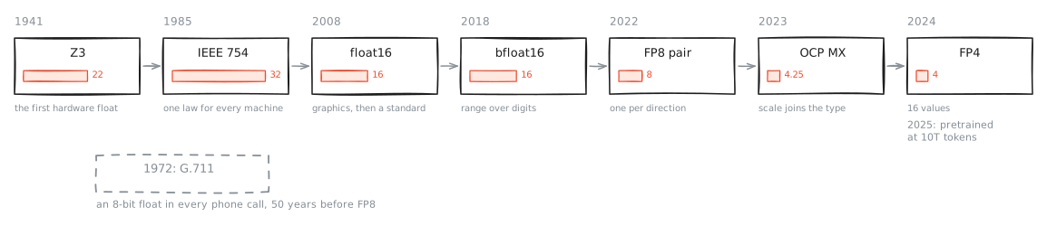
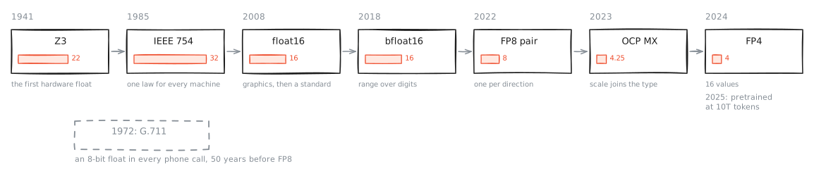
Konrad Zuse's Z3 computed in 22-bit floating point in 1941, special values included. 44 years later IEEE 754, largely William Kahan's design, ended an era in which every vendor's arithmetic disagreed [3]. The formats since bfloat16 are the same standard's ideas at new bit counts, and the full table of every named format that ever shipped, from the Z3 to the G.711 telephone float of 1972 (an 8-bit float in every phone call for 50 years) to NVFP4, is longer than this page and belongs to a follow-up table of its own. The roads not taken, posits and logarithmic number systems, are worth reading about [17].
Build it yourself
You already did, in the proofs. The 15-line decoder in p2_e4m3_map.py is a complete FP8 implementation that torch agrees with on all 256 patterns; the block quantizer in p11_mxblock.py is MXFP4 minus the packing; the stochastic rounder lives in p12_sr_drift.py. Change E4M3's constants to E5M2's and check yourself against torch again: that is the exercise that makes every format in this family yours.
p11_mxblock.py the proof, ready to read or run
download and run it# an mx-style block quantizer built from the spec.
#
# 32 elements share one power-of-2 scale (e8m0 has nothing but an
# exponent), elements are e2m1. the scale's exponent is rounded up,
# the choice that keeps the block maximum representable; the
# original ocp spec rounded down and lost it. then sweep block
# sizes to see the trade: scale overhead per element vs error.
import math, torch
E2M1 = torch.tensor([0.0, 0.5, 1.0, 1.5, 2.0, 3.0, 4.0, 6.0])
def round_e2m1(v):
idx = (v.abs().unsqueeze(-1) - E2M1).abs().argmin(-1)
return E2M1[idx] * v.sign()
def mx_quant(x, block=32):
q = torch.empty_like(x)
for i in range(0, len(x), block):
b = x[i:i+block]
amax = b.abs().max()
if amax == 0:
q[i:i+block] = 0; continue
e = math.ceil(math.log2(amax / 6.0)) # round up: amax stays <= 6 * 2^e
e = max(-127, min(127, e)) # e8m0's exponent range
s = 2.0 ** e
q[i:i+block] = round_e2m1(b / s) * s
return q
torch.manual_seed(1)
x = torch.randn(4096)
for block in (8, 16, 32, 64, 128):
q = mx_quant(x, block)
rel = ((q - x).abs() / x.abs().clamp_min(1e-9)).median()
bits = 4 + 8 / block # 4-bit element + 8-bit scale shared by the block
print(f"block {block:>3}: bits/element {bits:.3f} median rel err {rel:.1%}")
# and the rounding-direction subtlety, demonstrated on one block
b = torch.tensor([5.9] * 32)
e_up = math.ceil(math.log2(5.9 / 6.0)); e_dn = math.floor(math.log2(5.9 / 6.0))
up = round_e2m1(b / 2.0**e_up) * 2.0**e_up
dn = (round_e2m1((b / 2.0**e_dn).clamp(-6, 6)) * 2.0**e_dn)
print(f"\nblock of 5.9s: scale rounded up -> {up[0].item():.2f}, "
f"rounded down (clamped) -> {dn[0].item():.2f} (true 5.90)")
# the run prints (seeded):
#
# block 8: bits/element 5.000 median rel err 11.3%
# block 16: bits/element 4.500 median rel err 12.0%
# block 32: bits/element 4.250 median rel err 12.3%
# block 64: bits/element 4.125 median rel err 12.7%
# block 128: bits/element 4.062 median rel err 13.5%
#
# block of 5.9s: scale rounded up -> 6.00, rounded down (clamped) -> 3.00 (true 5.90)
#
# the sweep is the whole design argument for block = 32: going to 8
# costs 0.75 extra bits per element and buys 1 point of error;
# going to 128 saves 0.19 bits and gives 1.2 points back. and the
# last line shows why the rounding direction matters: round the
# scale's exponent the wrong way and a block full of 5.9s comes
# back as 3.0, off by nearly half.
What you can now say
- why 0.1 + 0.2 misses, and which 3 numbers were never stored
- how to convert 0.1 to binary by hand, and why its bits repeat
- what the exponent and mantissa each buy, what the bias is for, and why the leading 1 is never stored
- how to read any format's map: points per interval, step per interval, ulp, ceiling, floor, ramp
- every format's card: where it came from, where it runs, and the number at which it fails
- the whole family on one sheet: how the bits split between reach and digits, from float64's 2,098 doublings to FP4's 3.6
- why bfloat16 is float32's top 16 bits, at the bit level
- what absorption, cancellation and order-dependence do to real code, and which repair fits which
- every epsilon in a transformer, and the one-line softmax slide
- why training keeps a float32 master copy, and what loss scaling actually moves
- why FP8 is a pair, what a block scale is, why E8M0 has no mantissa, and why FP4 cannot live without blocks
- what stochastic rounding and Hadamard rotations buy at 4 bits
- why INT4, FP4 and NF4 put their 16 points in different places
- why two GPUs never agree to the last bit, why even a compiler's fusion choice can change a program's bits, and why neither is a bug
Try it yourself
Predict first, then run, then explain the difference: p0 the two opening questions; p1 your own histogram; p2 all 256 of E4M3; p4 absorption and cancellation; p5 order; p6 the cliff; p7 the fork; p8 the vanished update; p9 the slide; p10 the spike; p11 blocks; p12 stochastic rounding; p13 the rotation; p14 the three grids; p16 the four cards from two numbers; p17 all 65,536 bfloat16 patterns; p18 the family sheet; p19 one NVFP4 block by hand; p20 all 256 E5M2 patterns; p21 1 rounding against 2; p22 the error, caught exactly; p23 rounding twice. On paper: how many doublings separate E5M2's floor from its ceiling, and would the p1 gradients fit without a scale? And before running p16: derive float16's ceiling from E=5, M=10 yourself, the way the binary32 section taught you.
References
[1] Khalilli, proof scripts for this page, measured on an Apple M3 Max, torch 2.11.0, CPU, 2026. Linked in place above; rerun them to check me.
[2] Sanglard, Floating Point Visually Explained, 2017. The interval-and-position way of seeing the fields comes from here. https://fabiensanglard.net/floating_point_visually_explained/
[3] IEEE, 754-2019: Standard for Floating-Point Arithmetic (first edition 1985).
[4] Goldberg, What Every Computer Scientist Should Know About Floating-Point Arithmetic, ACM Computing Surveys, 1991; and Muller et al., Handbook of Floating-Point Arithmetic, 2nd ed., 2018.
[5] Micikevicius et al., Mixed Precision Training, ICLR 2018. https://arxiv.org/abs/1710.03740
[6] Micikevicius et al., FP8 Formats for Deep Learning, 2022. https://arxiv.org/abs/2209.05433
[7] DeepSeek-AI, DeepSeek-V3 Technical Report, 2024. https://arxiv.org/abs/2412.19437
[8] Dettmers et al., LLM.int8(): 8-bit Matrix Multiplication for Transformers at Scale, 2022 (the emergent-outlier measurement). https://arxiv.org/abs/2208.07339
[9] Open Compute Project, Microscaling Formats (MX) Specification v1.0, 2023; and Rouhani et al., Microscaling Data Formats for Deep Learning, 2023. https://arxiv.org/abs/2310.10537
[10] NVIDIA, Pretraining Large Language Models with NVFP4, 2025. https://arxiv.org/abs/2509.25149
[11] Mishra et al., Recipes for Pre-training LLMs with MXFP8, 2025 (the scale-rounding result). https://arxiv.org/abs/2506.08027
[12] Tseng et al., Training LLMs with MXFP4, 2025. https://arxiv.org/abs/2502.20586
[13] Dettmers et al., QLoRA: Efficient Finetuning of Quantized LLMs, 2023 (NF4). https://arxiv.org/abs/2305.14314
[14] Frantar et al., GPTQ, 2022. https://arxiv.org/abs/2210.17323
[15] Lin et al., AWQ: Activation-aware Weight Quantization, 2023. https://arxiv.org/abs/2306.00978
[16] Dettmers et al., 8-bit Optimizers via Block-wise Quantization, 2021. https://arxiv.org/abs/2110.02861
[17] Gustafson and Yonemoto, Beating Floating Point at its Own Game: Posit Arithmetic, 2017; logarithmic number systems survey in Muller et al. [4].
[18] Severance, An Interview with the Old Man of Floating-Point (William Kahan on IEEE 754 and the Intel 8087), 1998. https://people.eecs.berkeley.edu/~wkahan/ieee754status/754story.html
[19] NVIDIA, CUDA C++ Programming Guide, the arithmetic instructions throughput table (per-architecture float64 rates). https://docs.nvidia.com/cuda/cuda-c-programming-guide/
[20] Kharya, TensorFloat-32 in the A100 GPU Accelerates AI Training, HPC up to 20x, NVIDIA blog, 2020. https://blogs.nvidia.com/blog/tensorfloat-32-precision-format/
[21] PyTorch documentation, CUDA semantics (the TF32 flags and their defaults since 1.12). https://docs.pytorch.org/docs/stable/notes/cuda.html
[22] Industrial Light & Magic, About OpenEXR (the half type, 2000-2003, and its Cg compatibility); and Bogart, Kainz, Hess, The OpenEXR Image File Format, GPU Gems, 2004. https://openexr.com/en/latest/about.html
[23] Wang and Kanwar, BFloat16: The secret to high performance on Cloud TPUs, Google Cloud blog, 2019. https://cloud.google.com/blog/products/ai-machine-learning/bfloat16-the-secret-to-high-performance-on-cloud-tpus
[24] Ku, Poli et al. (Radical Numerics), NVFP4 pretraining: from theory to implementation, Part 1, 2026. The recipe walk-through this page's NVFP4 worked block follows. https://www.radicalnumerics.ai/blog/nvfp4-part1
[25] Easygoing, Which is Better: FP8_scaled or MXFP8? A Thorough Comparison of Image Generation AI Model Accuracy and Speed, AI Image Journey, 2026. The measured quality ranking and the measured slowdown of MXFP8 on hardware without MX support. https://note.com/ai_image_journey/n/n99d0ed2f1c1d
[26] ZeroEntropy, MXFP4 (concepts), 2026. The per-vendor native-support summary. https://zeroentropy.dev/concepts/mxfp4/
[27] Boehm, Can Function Inlining Affect Floating Point Outputs? Exploring FMA and Other Consistency Issues, 2023. https://siboehm.com/articles/23/Inlining-FMA-FP-consistency
[28] PyTorch documentation, Numerical accuracy. https://docs.pytorch.org/docs/stable/notes/numerical_accuracy.html
[29] Kwon et al., Efficient Memory Management for Large Language Model Serving with PagedAttention (the vLLM paper), 2023. https://arxiv.org/abs/2309.06180
[30] NVIDIA, H100 Tensor Core GPU specifications (HBM3 bandwidth and PCIe generation 5 rates). https://www.nvidia.com/en-us/data-center/h100/
[31] He and Thinking Machines Lab, Defeating Nondeterminism in LLM Inference, Connectionism, 2025. The 1,000-completions measurement and the batch-invariant kernels. https://thinkingmachines.ai/blog/defeating-nondeterminism-in-llm-inference/
Three good things to read after this page: Goldberg's paper [4] slowly, with the map in hand; the OCP MX specification [9], which is short and readable; and Kahan's interview on the making of IEEE 754 [18], where the standard's designer tells the story himself.